
I started this question over at Biostars (https://www.biostars.org/p/341052/) , and I did get help and applied some suggestions from the community over there. However, I still have some remaining doubts, and maybe I should have come here first since it seems it is indeed an issue of how I'm using DESeq2 rather than previous points in the RNAseq analysis.
Quick summary: We are working on a non-model organism, with no genome or transcriptome databases. We are analyzing 4 tissues under 2 treatments, each one in triplicate. The pipeline goes as such: trinity -> salmon -> tximport -> deseq2. We want to use a common pipeline for both transcript and 'gene' level, so that's the reason behind the choice of DESeq2. Below is creating the object for transcript level comparisons.
txi.salmon <- tximport(files, type= 'salmon', countsFromAbundance= 'scaledTPM', txOut=TRUE, dropInfReps=TRUE)
colDesign <- data.frame(row.names=samples$sample, tissue=samples$tissue, diet=samples$diet, replicate=samples$replicate )
dds <- DESeqDataSetFromTximport(txi.salmon, colData=colDesign, design= ~tissue+diet)
dds$group <- factor(paste0(dds$diet,dds$tissue))
design(dds) <- ~group
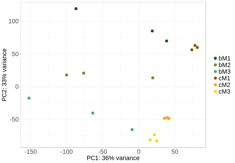
The odd thing about the results comes when looking at the fold changes and right-skewed hill p-value distributions of the contrasts. Before any correction I was getting plots that showed that no small log2 fold change, usually around -2 to 2, was flagged as significant, and also getting some truly remarkable fold changes of 50 or so. By inspection of the PCA plot, one of the suggestions was to rerun without samples from one of the tissues as it clusters far from the other three tissues. The new PCA shows the two treatments do not have the same dispersion, with C clustering tightly and B more spread out.
I read that DESeq2's single dispersion parameter might not be adequate in this situation, and to use the fdrtool package to re estimate the null model. This did flatten out the expected p-value distributions (my call of contrast does not use the lfcThreshold and altHypothesis arguments), but it drastically elevated the number of transcripts identified as significant (sometimes from a few hundreds to tens of thousands). Thinking the low count non-informative transcripts from the assembly are contributing to these changes, I wanted to apply the shrinkage to the log folds. The TPM of the vast majority of transcripts in the assembly is indeed below 10. I ended up using betaPrior=TRUE when running DESeq because for some reason using lfcshrink() on the extracted results never finished. I understand this changes how the p-values are computed.
In essence, I want to know if it is statistically sound to use these different modifications together:
- shrinkage to control for the wide changes in low count transcripts
- alternative hypothesis to test for biologically relevant fold change rather than the small, but significant ones with the default null hypothesis
- re-estimating the null model due to differences in dispersion between the two treatments.
I don't know if it would be overcorrecting too much, or the type of results I'm seeing is expected with DESeq2 given the type of dataset I'm working with.
Also, the output of sessionInfo()
R version 3.4.4 (2018-03-15)
Platform: x86_64-pc-linux-gnu (64-bit)
Running under: Ubuntu 18.04.1 LTS

Matrix products: default
BLAS: /usr/lib/x86_64-linux-gnu/blas/libblas.so.3.7.1
LAPACK: /usr/lib/x86_64-linux-gnu/lapack/liblapack.so.3.7.1

locale:
 [1] LC_CTYPE=en_US.UTF-8       LC_NUMERIC=C               LC_TIME=en_US.UTF-8        LC_COLLATE=en_US.UTF-8     LC_MONETARY=en_US.UTF-8
 [6] LC_MESSAGES=en_US.UTF-8    LC_PAPER=en_US.UTF-8       LC_NAME=C                  LC_ADDRESS=C               LC_TELEPHONE=C
[11] LC_MEASUREMENT=en_US.UTF-8 LC_IDENTIFICATION=C

attached base packages:
[1] parallel  stats4    stats     graphics  grDevices utils     datasets  methods   base

other attached packages:
 [1] fdrtool_1.2.15             geneplotter_1.56.0         annotate_1.56.2            XML_3.98-1.16              AnnotationDbi_1.40.0
 [6] lattice_0.20-35            ggplot2_3.0.0              BiocParallel_1.12.0        readr_1.1.1                tximport_1.6.0
[11] DESeq2_1.18.1              SummarizedExperiment_1.8.1 DelayedArray_0.4.1         matrixStats_0.54.0         Biobase_2.38.0
[16] GenomicRanges_1.30.3       GenomeInfoDb_1.14.0        IRanges_2.12.0             S4Vectors_0.16.0           BiocGenerics_0.24.0

loaded via a namespace (and not attached):
 [1] bit64_0.9-7            splines_3.4.4          Formula_1.2-3          assertthat_0.2.0       latticeExtra_0.6-28    blob_1.1.1
 [7] GenomeInfoDbData_1.0.0 yaml_2.2.0             pillar_1.3.0           RSQLite_2.1.1          backports_1.1.2        glue_1.3.0
[13] digest_0.6.17          RColorBrewer_1.1-2     XVector_0.18.0         checkmate_1.8.5        colorspace_1.3-2       htmltools_0.3.6
[19] Matrix_1.2-14          plyr_1.8.4             pkgconfig_2.0.2        genefilter_1.60.0      zlibbioc_1.24.0        purrr_0.2.5
[25] xtable_1.8-3           scales_1.0.0           htmlTable_1.12         tibble_1.4.2           withr_2.1.2            nnet_7.3-12
[31] lazyeval_0.2.1         survival_2.42-6        magrittr_1.5           crayon_1.3.4           memoise_1.1.0          foreign_0.8-71
[37] tools_3.4.4            data.table_1.11.8      hms_0.4.2              stringr_1.3.1          locfit_1.5-9.1         munsell_0.5.0
[43] cluster_2.0.7-1        bindrcpp_0.2.2         compiler_3.4.4         rlang_0.2.2            grid_3.4.4             RCurl_1.95-4.11
[49] rstudioapi_0.8         htmlwidgets_1.3        bitops_1.0-6           base64enc_0.1-3        gtable_0.2.0           DBI_1.0.0
[55] R6_2.3.0               gridExtra_2.3          knitr_1.20             dplyr_0.7.6            bit_1.1-14             bindr_0.1.1
[61] Hmisc_4.1-1            stringi_1.2.4          Rcpp_0.12.19           rpart_4.1-13           acepack_1.4.1          tidyselect_0.2.4

We are interested in comparing between tissues within one treatment (so, G tissue versus M1, G tissue vs M2, M1 vs M2, etc) and between the same tissue but with different treatment, which is where the dispersions vary. I should note that even when contrasting one M tissue to another within one treatment, the p-value distribution was also skewed, so that confuses me as well as to why I'm getting these results. EDIT: I went back to confirm this. It is true, but once I plot only those with base mean 20 or more it flattens out. It is kind of giving me an idea of the actual cutoff for filtering that will be useful.
For shrinkage, I saw in the vignette that to use apeglm and extract results one uses the coef argument, rather than contrast, and that ashr does not work with the lfcThreshold argument. I wasn't sure how that would affect the results, so I was changing just one parameter at a time and stuck with the "normal" shrinkage. I also wasn't sure how to use the coef argument. The results object generated with the ~group design as above didn't list all the comparisons I was interested in with resultsNames(), so I don't how to specify them to the function. I might just do what you recommend and create separate dds with the samples for each set of pairwise comparisons.
So if you compare two groups within 'b' or 'c' above, there is a skew to the p-value histogram (aside from a spike at 0)?
For apeglm, if you run with just two groups of samples at a time (recommended given the PCA above), you would set coef=2.
If I use all 24 samples and compare tissues within treatment, and plot by filtering those with low base mean, there is only a slight right skew, and no peaks besides the one at 0. It looks as expected for the test. It is only when comparing the same tissue between C and B that the distributions skew to the right, and can't recover a regular flat plot no matter how much I fiddle around.
If I construct and test the dds object with just the samples from one treatment, I start getting right skews in the p-value distributions no matter how I plot the data, which seems counter-intuitive to what the PCA would suggest. It's the same if I construct and test the dds object in a pairwise way, although slightly less pronounced. I have the feeling I just have one truly pathologic expression dataset. Of note: using apeglm apparently produces some even weirder volcano plots than what I was seeing originally. I will keep testing.
By the way, if you are using lfcThreshold, the p values are not supposed to be uniform anymore. You didn’t post the code where you run DESeq() or results(), but I wanted to add that. Our implementation of the threshold test is conservative (see Methods section of the paper) which means the right skew is expected and should definitely not be corrected with any modification of the p values.
I will expand a little on my previous replies with graphs, I hope it clears up the situation. I'm running DESeq in the following way:
At first I was using just variations the following code to get the contrasts with the dds object with the 24 samples:
res_cM1_vs_cM3 <-results(de_results,contrast=c('group','cM1','cM3'),alpha=0.05)
and the p-value distribution looked like this:
If I do the same but add the LFC threshold parameter the p-value distribution turns into this:
res_cM1_vs_cM3 <-results(de_results,contrast=c('group','cM1','cM3'), alpha=0.05 ,lfcThreshold = 1, altHypothesis = 'greaterAbs')This is representative. Most contrasts looked similar or quite worse before changing the null hypothesis. The right skew is even higher if I build dds with pairwise samples according to the PCA, though it also changes by adding the LFC threshold.
I hadn't been using the lfcThreshold in conjunction with shrinking, just to have a better idea of how the data behaved, but seeing as it seems to be more appropriate, I would need to use apeglm, not ashr, to do it from what I read in the vignette. When I do use apeglm with coef=2 as you suggested, it's having some very weird effects on the data, for example when plotting fold change vs p-adj.
original (24 samples)
pairwise
pairwise shrunk
hi Emiliano,
Thanks for these plots. The LFC threshold distribution is just as you would expect. the spike near 1 is from the genes where the LFC lies within the zone you have defined as null. They have high p-values. So don't expect that the dist'n of p-values will be uniform with lfcThreshold.
Regarding apeglm here, it is being a lot more conservative in the point estimate than DESeq2's p-values. I suppose it's not consistent with the p-values and adjusted p-values, as it's being so much more conservative (it's perhaps more responsive to the high inter-group variance you see in the PCA plot above). That may argue for using type="normal" on this dataset, I suppose.
Thank for all your suggestions, Michael. Dealing with the de novo transcriptomes is always messier than having a reference. In my previous projects I've dealt with more studied organisms, so this dataset has proven a bit trickier to tackle.
For the shrinking methods, I'm not sure what you mean. The image I showed is from a pairwise comparison of two groups that, at least by the PCA, look to have similar within group variance (cM1 and cM3). After inspecting results I realize I will need to implement shrinking of some kind. Some of the highly significant transcripts with very high fold changes are some that have have low counts (or zeroes in almost all samples) .
I see. Then maybe apeglm is preferred. If you use lfcThreshold with apeglm you will produce svalues that are consistent with the point estimates.