Hi, I am trying to help a labmate who is using DiffBind to do a PCA analysis on some ATAC-seq data that she generated. I have experience with PCA but not with this specific software. How can we retrieve the PCA loadings/eigenvalues for each individual for each PC? I am used to using other PCA tools that allow you to retried the spreadsheet of loadings/eigenvalues in addition to plotting PC's 1-10 against each other. As far as I can tell DiffBind allows you to plot PC1, PC2, and PC3 against each other but does not provide the actual numbers, nor does it provide access to any further PC's. Any help with this would be greatly appreciated.
Wanted to do something similar and indeed was unable to find PCA loadings. However I did find that plotting dba.plotPCA(dba, DBA_ID) and dba.plotPCA(dba, DBA_TREATMENT) (so by sample ID and treatment group, respectively), I was able to see which sample corresponds to which in the treatment PCA plot. So not exact eigenvalues as you wanted, but you can at least get an idea of which samples cluster together/away from each other which is all I was trying to do at the end of the day.
DiffBind does allow any components to be plotted again any other components by specifying which components to plot using components= when calling dba.plotPCA() (the default is components=1:3 but this may be changed by the user).
There is no way to directly retrieve the computed PCA data. You can retrieve the underlying read count data (normalized by default) using dba.peakset() with bRetrieve=TRUE and run a PCA on that.
Thanks Rory!! In future versions of the software it might be helpful to be able to retrieve the computed PCA data, but this will work. :) Thanks for your quick response!!
Note that by default DiffBind does PCA using log2() values.
I should also mention that if you are looking to get the counts for differentially bound sites only, you can call dba.report() with bCounts=TRUE and form a matrix with the count metadata columns.
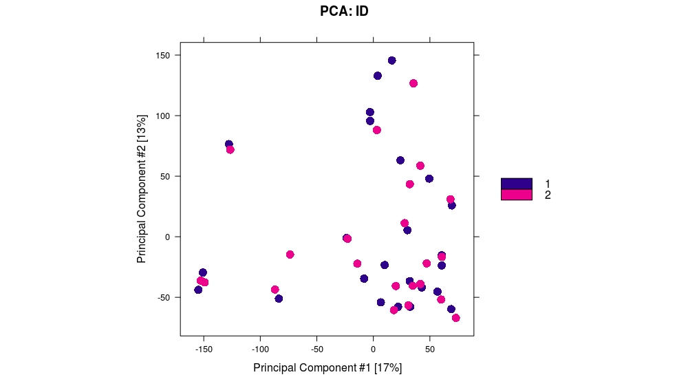
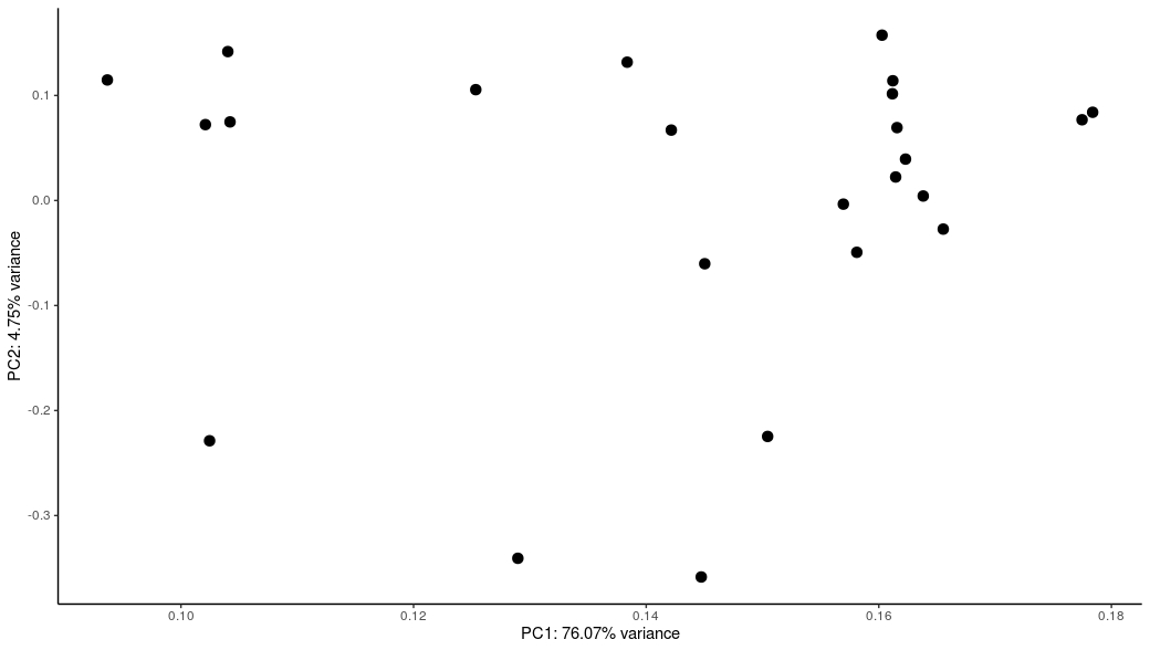
For my dataset, I have a hard time to reproduce the result from dba.plotPCA(dba), but the proportion of variance is way off ( 17% from dba.plotPCA vs 76% from the following code for PC1). I try different score but the % remain similar. Also the x and y-axis scale are different too (screenshot attached).
Also, following the instruction from an older post:


Wanted to do something similar and indeed was unable to find PCA loadings. However I did find that plotting dba.plotPCA(dba, DBA_ID) and dba.plotPCA(dba, DBA_TREATMENT) (so by sample ID and treatment group, respectively), I was able to see which sample corresponds to which in the treatment PCA plot. So not exact eigenvalues as you wanted, but you can at least get an idea of which samples cluster together/away from each other which is all I was trying to do at the end of the day.