Dear List and Professor Smyth,

I would like to process my Nanostring GeoMX spatial data using limma. I am working with normalized data output from the Nanostring software names "Q3 TargetCountMatrix". According to the Nanostring user guide (MAN-10119-01_GeoMx-NGS_Data_Analysis_User_Manual.pdf)

"Q3 (3rd quartile of all selected targets) is the recommended normalization method for NGS data for all targets that are above the limit of quantitation (LOQ). Q3 normalization uses the top 25% of expressers to normalize across ROIs/segments, so it is robust to changes in expression of individual genes and ideal for making comparisons across ROIs/segments."

This produces a spreadsheet of targets (gene names) and non-integer expression data. I think it would be good to process this data with limma as the nanostring data analysis methods are not as ideal. What I would like to know is if this is a good idea. Any info or feedback is greatly appreciated.

library(limma)

# Import the Q3 Nanostring data
dat <- read.csv("29Jun21_WS_nanostring.csv", sep="\t", header=T)
rownames(dat) <- dat$GeneID

# Subset the data
keeps <- c("WT_V1", "WT_V2", "WT_V3", "WT_V4", "WT_V5", "KO_NV1", "KO_NV2", "KO_NV3")
data < dat[keeps]

# log base 2 transform
md1 <- as.matrix(log2(data))

# Normalize the data (Is there a better way to do this?? Is this cool to do?)
mdn <- normalizeBetweenArrays(md1, method="cyclicloess", cyclic.method="affy")

# Boxplot doesn't look terrible![boxplot][1]
boxplot(as.data.frame(mdn),main="Cyclic Loess Normalization Affy-style")

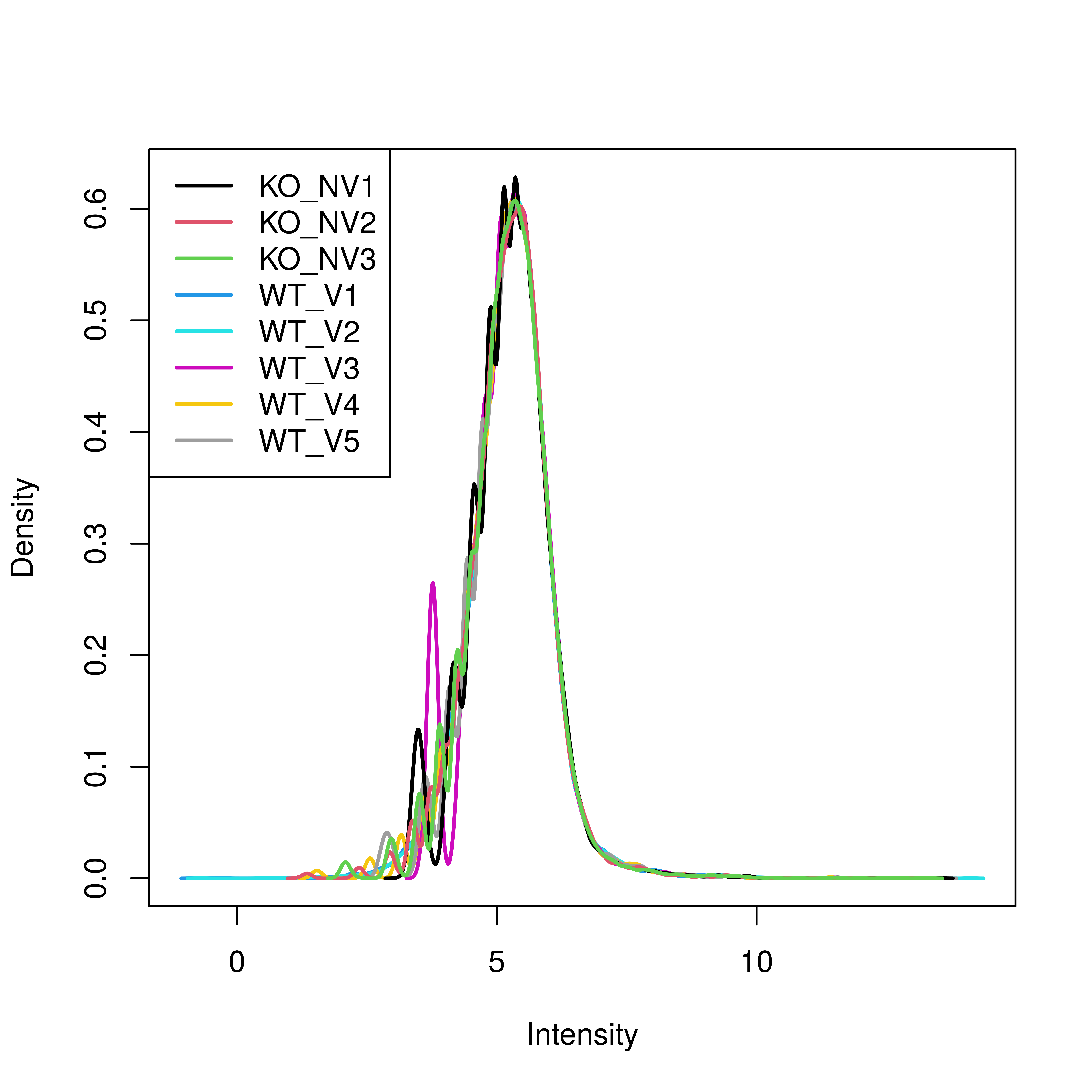
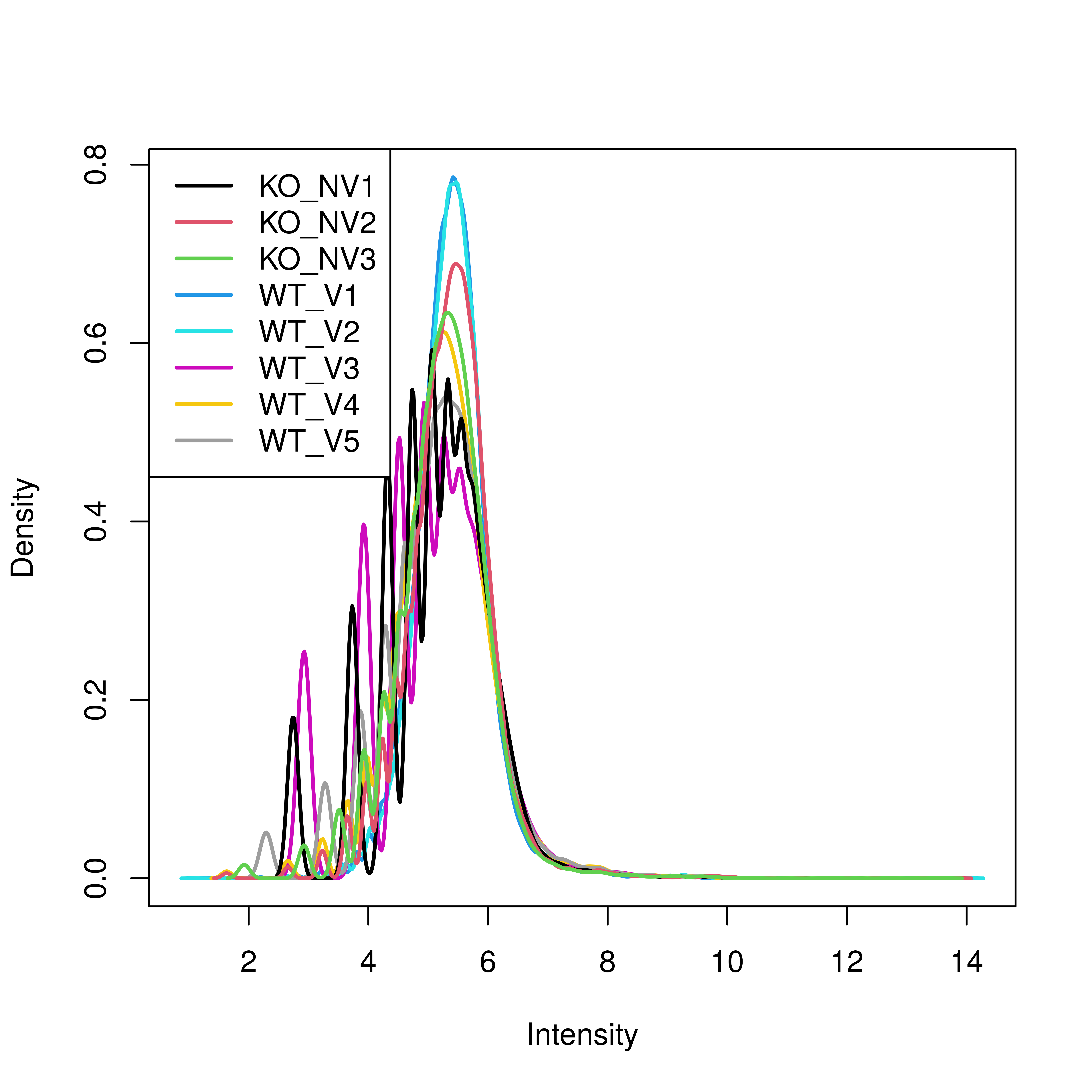
# Density plot is not as smooth as it could be.  It is smooth past the peak. 'Affy' cyclic loess was the strongest.
plotDensities(mdn)

  # Perform the DE testing
    group <- factor(c("CTR", "CTR", "CTR", "CTR", "CTR", "KO", "KO", "KO"))
    design <- model.matrix(~0 + group)

    fit <- lmFit(mdn, design)
    contr <- makeContrasts(groupKO - groupCTR, levels = colnames(coef(fit)))

fit2 <- contrasts.fit(fit, contr)

fit3 <- eBayes(fit2)

# Not too many DE genes
summary(decideTests(fit3))

# Get the data out
top <- topTable(fit3, sort.by = "B", n = Inf)

sessionInfo( )
R version 4.0.3 (2020-10-10)
Platform: x86_64-pc-linux-gnu (64-bit)
Running under: Ubuntu 18.04.5 LTS

Matrix products: default
BLAS/LAPACK: /usr/local/lib/OpenBLAS/OpenBLAS-0.2.20/build/lib/libopenblas_nehalemp-r0.2.20.so

locale:
 [1] LC_CTYPE=en_US.UTF-8       LC_NUMERIC=C              
 [3] LC_TIME=en_US.UTF-8        LC_COLLATE=en_US.UTF-8    
 [5] LC_MONETARY=en_US.UTF-8    LC_MESSAGES=en_US.UTF-8   
 [7] LC_PAPER=en_US.UTF-8       LC_NAME=C                 
 [9] LC_ADDRESS=C               LC_TELEPHONE=C            
[11] LC_MEASUREMENT=en_US.UTF-8 LC_IDENTIFICATION=C       

attached base packages:
[1] parallel  stats     graphics  grDevices utils     datasets  methods  
[8] base     

other attached packages:
[1] gplots_3.1.1        marray_1.68.0       limma_3.46.0       
[4] Biobase_2.50.0      BiocGenerics_0.36.1

loaded via a namespace (and not attached):
 [1] pillar_1.6.1          compiler_4.0.3        BiocManager_1.30.16  
 [4] bitops_1.0-7          tools_4.0.3           zlibbioc_1.36.0      
 [7] preprocessCore_1.52.1 lifecycle_1.0.0       tibble_3.1.2         
[10] gtable_0.3.0          lattice_0.20-44       pkgconfig_2.0.3      
[13] rlang_0.4.11          DBI_1.1.1             dplyr_1.0.7          
[16] generics_0.1.0        vctrs_0.3.8           gtools_3.9.2         
[19] caTools_1.18.2        grid_4.0.3            tidyselect_1.1.1     
[22] glue_1.4.2            R6_2.5.0              fansi_0.5.0          
[25] ggplot2_3.3.5         purrr_0.3.4           magrittr_2.0.1       
[28] scales_1.1.1          ellipsis_0.3.2        assertthat_0.2.1     
[31] colorspace_2.0-2      utf8_1.2.1            KernSmooth_2.23-20   
[34] affy_1.68.0           munsell_0.5.0         vsn_3.58.0           
[37] crayon_1.4.1          affyio_1.60.0        

```