GSVA and ssGSEA output differences
1
0
Entering edit mode
Davide • 0
@a00f114c
Last seen 10 months ago
Italy

Hi everyone,

I have a question about the GSVA package, In particular about the results with different methods parameter value ("ssGSEA" and "GSVA" ). In my case I have 5 sample and I want to test the enrichment of 2 genesets on them. The step of my analysis was the following:

  • produce a raw counts matrix for BAM files
  • normalise the raw counts (DESeq2)
  • transform the normalised counts via regularised log
  • Run GSVA

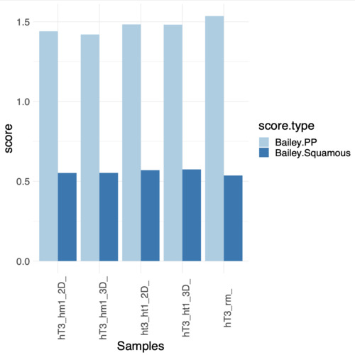
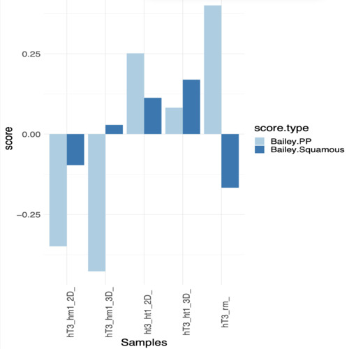
I've performed the gsva() 2 times with same parameter except for the method; one time i used ssGSEA and for the other GSVA, the results i've obtained led to opposite conclusions (regarding the enrichment of the two genesets). I've attached the plot showing the obtained scores

enter image description hereenter image description here On the left GSVA score plot and ssGSEA on the right.

My question is, it's possible that the two methods gives me such opposite results when described as "similar" in the help page? I've read the reference paper trying to understand better which could be the source of the variation but i think i'm loosing something (or more), it's probably due to the gene ranking step? even if it's due to that or from other aspects of the computation i didn't expect, from what i know, such a difference in results. If someone can fill my gap in knowledge for big it is and give me some insights/explanations on the argument and results understanding it would be awesome. Let me know if more information are needed from me on the problem.

enrichment GSVA enrichplot ssGSEA • 5.3k views
ADD COMMENT
0
Entering edit mode
Robert Castelo ★ 3.3k
@rcastelo
Last seen 1 day ago
Barcelona/Universitat Pompeu Fabra

hi,

GSVA is similar to ssGSEA in that it is a non-parametric method that uses the empirical CDFs of gene expression ranks inside and outside the gene set, but it has some features that make it different to ssGSEA. The fact that all your ssGSEA scores are positive while GSVA scores are positive and negative suggests to me that there could be some problem in the way you are calling both methods, some unintended error, but I would need to access the data and the code that you use to be able to tell you more about where these differences come from. Another way in which you may check the extent to which the results make sense is by exploring the expression values of the genes that form each gene set. For a positive GSVA score, the genes forming the gene set should have a higher expression that the genes forming a gene set with a negative GSVA score.

ADD COMMENT
0
Entering edit mode

Hi, Thanks for the reply, i looked at the genes expressions data and i have an idea which result have more sense. At the same time i'm posting here data and code, if you have time to look at that, it will be awesome.

here the data: https://univr-my.sharepoint.com/:u:/g/personal/davide_pasini_univr_it/EaPXg7f2LrFLlXId8JoKSSkBKhhUwoeqTBMrjdW4MW_n6Q?e=fmKA1G[ link]1

here a trimmed version of the code i used, with the main workflow:

library(GSVA)
library(DESeq2)
library(stringr)
library(msigdbr)
library(ggplot2)
library(plyr)

#Functions
addScore <- function(matrix , list = NULL, max = Inf, min = -Inf, method = "gsva"){
  print(method)
  gs = gsva(expr = assay(matrix), list, min.sz = min, max.sz = max, method = method)
  print(head(gs))
  colData(matrix) = cbind(colData(matrix), t(gs))

  return(matrix)
}

converter <- function(x, type = "ENS"){
  require("biomaRt")
  human = useMart("ensembl", dataset = "hsapiens_gene_ensembl")
  mouse = useMart("ensembl", dataset = "mmusculus_gene_ensembl")

  switch(type,
         ENS = {
           genesV2 = getLDS(attributes = c("ensembl_gene_id"),
                            filters =  "ensembl_gene_id",
                            values = x,
                            mart = mouse,
                            attributesL = c("ensembl_gene_id"),
                            martL = human, uniqueRows = T)
         },
         SYMB = {
           genesV2 = getLDS(attributes = c("mgi_symbol"),
                            filters = "mgi_symbol",
                            values = x ,
                            mart = mouse,
                            attributesL = c("hgnc_symbol"),
                            martL = human, uniqueRows=T)
         },

         Human_ENS_SYMB = {
           genesV2 = getBM(attributes='hgnc_symbol', 
                 filters = 'ensembl_gene_id', 
                 values = x, 
                 mart = human ,uniqueRows=T)
         },
         Human_SYMB_ENS = {
           genesV2 = getBM(attributes = 'ensembl_gene_id', 
                           filters = 'hgnc_symbol', 
                           values = x, 
                           mart = human,uniqueRows=T)
         }
  )
  print(head(genesV2))
  return(genesV2)
}

#main code
counts = read.table("./merged_results_on_geneID.txt")

counts$gene_id = unlist(lapply(str_split(counts$gene_id, pattern = "\\."),'[',1))
counts = ddply(counts, "gene_id", numcolwise(sum))
rownames(counts) = counts$gene_id
counts$gene_id = NULL

colnames(counts) = lapply(lapply(stringr::str_split(colnames(counts), pattern = "_"),'[',c(1:4)),paste0,sep="_",collapse="")
coldata = as.data.frame(colnames(counts))
rownames(coldata) = colnames(count)
for (i in colnames(counts)) {
  counts[,i] = as.integer(counts[,i])

 }

dds = DESeqDataSetFromMatrix(counts, design = ~1, colData = coldata)

nrow(dds)
#keep <- rowSums(counts(RNA_table) >= 1) >= 21
keep <- rowSums(counts(dds)) > 1
table(keep)
RNA_filt <- dds[keep,]
nrow(RNA_filt)

RNA_filt2 <- DESeq(RNA_filt)

RNA_rl<- rlog(RNA_filt2)

Bailey = readRDS("Bailey_sig.Rds")

##########################
######### GSVA ###########
##########################

RNA_rl = addScore(matrix =  RNA_rl, list = Bailey, min = 5)

############################
######### ssGSEA ###########
############################

RNA_rl = addScore(matrix =  RNA_rl, list = Bailey, min = 5, method = "ssgsea")
ADD REPLY
1
Entering edit mode

ok, from what i see both results, GSVA and ssGSEA are quite proportional to each other, if you rename the objects that get the result in the last two calls from the previous code, to dseqobj_gsva and dseqobj_ssgsea, respectively, and you plot them doing:

plot(dseqobj_gsva$Bailey.PP, dseqobj_ssgsea$Bailey.PP)
plot(dseqobj_gsva$Bailey.Squamous, dseqobj_ssgsea$Bailey.Squamous)

you should see what i'm talking about, they are linearly correlated with each other with rho about 0.95. The difference is in the scale of values that you get from each method. In any case, you say you have an idea which result make more sense to you, so that should help you decide how do you want to do your analysis.

As a side note, I notice that after filtering lowly expressed genes, you still keep about 24,000, this is I think way too many because usually only about the half are expressed in a given experimental condition, tissue, etc. If you look at the distribution of average expression values per gene by doing:

hist(rowMeans(assay(RNA_rl)))

You will still see two well separated modes, the one on the left is made of genes that are probably not reliably expressed. I'd suggest to remove those.

ADD REPLY

Login before adding your answer.

Traffic: 760 users visited in the last hour
Help About
FAQ
Access RSS
API
Stats

Use of this site constitutes acceptance of our User Agreement and Privacy Policy.

Powered by the version 2.3.6