Using SingleR for Single cell annotation with BulkRNASeq
2
0
Entering edit mode
@rohitsatyam102-24390
Last seen 5 weeks ago
India

Hi Aaron.

I have Time-series bulk data (with two biological replicates for each time) and now I wish to use it to annotate my single-cell data. My Single-cell data contains two samples, One control and one drug-treated.

Your vignette is quite straight forward but can you tell me how I combine two biological replicates per time point into one column so that I have one column for each time point and use it for assigning labels. Will log normalizing both replicates and then take average per gene per time point work?

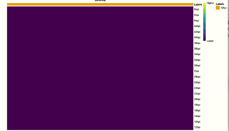
Update1: I actually did it as I mentioned above and used the following code. My cells are highly synchronized at 10 hours post-infection and I was using Bulk RNASeq to confirm the same using SingleR. But I am getting score 1 for all the time points. However, the final label assigned is correct i.e 10hpi. Weird though that the heatmap is all blue not yellow!!

library(SingleR)
library(Seurat)
library(dplyr)
c <- read.csv("../time_series_data/counts.csv", header = T, row.names = 1)
> c %>% head()
              T0_rep1 T0_rep2 T2_rep1 T2_rep2 T4_rep1 T4_rep2 T6_rep1
Gene1      46      48     202     298     357     428     125
Gene2     130     137     693     844    1713    1504     630
Gene3       0       0       0       0       1       0       0
Gene4       1       1       1       0       0       1       1
Gene5     412     524     994    1569    1959    2095     771
Gene6   16909   16966   16490   23660   30364   30484   10008

meta <- read.csv("../time_series_data/meta.csv", header = T)
> meta %>% head()
        Sample_id Prefix Replicate Time timetag
T0_rep1   T0_rep1     T0      rep1    4    4hpi
T0_rep2   T0_rep2     T0      rep2    4    4hpi
T2_rep1   T2_rep1     T2      rep1    6    6hpi
T2_rep2   T2_rep2     T2      rep2    6    6hpi
T4_rep1   T4_rep1     T4      rep1    8    8hpi
T4_rep2   T4_rep2     T4      rep2    8    8hpi

rownames(meta) <- meta$Sample_id
bulk <- CreateSeuratObject(counts = c, project = "Time-Series")
bulk$Sample <- "T-series"
bulk$batch <- "T-series"
bulk$batch2 <- "T-series"
bulk@meta.data <- cbind(bulk@meta.data,meta)
bulk <- NormalizeData(bulk)
prefix <- unique(meta$Prefix)
mat.temp <- data.frame(GetAssayData(bulk, slot="data"))
l <- list()
biorepavg <- lapply(1:length(prefix),function(x){
  l[[x]] <- mat.temp[,grep(prefix[x], colnames(mat.temp))] %>% rowMeans()

  })

df <- data.frame(sapply(biorepavg,c))
colnames(df) <- prefix
newmeta <- meta[,c(2,4,5)] %>% unique() %>% `rownames<-`(.$Prefix)
> newmeta %>% head
    Prefix Time timetag
T0      T0    4    4hpi
T2      T2    6    6hpi
T4      T4    8    8hpi
T6      T6   10   10hpi
T8      T8   12   12hpi
T10    T10   14   14hpi
tseries <- SingleCellExperiment(list(logcounts=df),colData=DataFrame(label=newmeta))
> pred.10nt.ts <- SingleR(test=p10NT.sce, ref=tseries, labels=tseries$label.timetag, de.method="wilcox",de.n=20)

> pred.10nt.ts$scores %>% head()
     10hpi 12hpi 14hpi 16hpi 18hpi 20hpi 22hpi 24hpi 26hpi 28hpi 2hpi
[1,]     1     1     1     1     1     1     1     1     1     1    1
[2,]     1     1     1     1     1     1     1     1     1     1    1
[3,]     1     1     1     1     1     1     1     1     1     1    1
[4,]     1     1     1     1     1     1     1     1     1     1    1
[5,]     1     1     1     1     1     1     1     1     1     1    1
[6,]     1     1     1     1     1     1     1     1     1     1    1
     30hpi 32hpi 34hpi 36hpi 38hpi 40hpi 42hpi 44hpi 4hpi 6hpi 8hpi
[1,]     1     1     1     1     1     1     1     1    1    1    1
[2,]     1     1     1     1     1     1     1     1    1    1    1
[3,]     1     1     1     1     1     1     1     1    1    1    1
[4,]     1     1     1     1     1     1     1     1    1    1    1
[5,]     1     1     1     1     1     1     1     1    1    1    1
[6,]     1     1     1     1     1     1     1     1    1    1    1

> pred.10nt.ts$labels %>% head()
[1] "10hpi" "10hpi" "10hpi" "10hpi" "10hpi" "10hpi"

enter image description here

SingleR • 1.7k views
ADD COMMENT
0
Entering edit mode

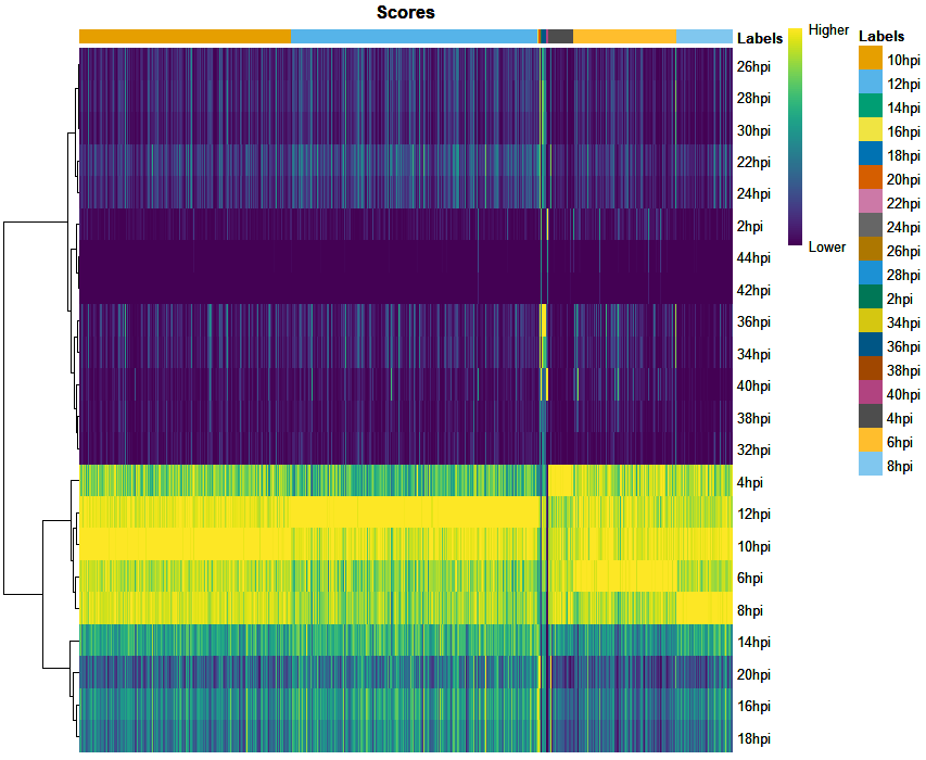
UPDATE 2: Repeated the analysis after removal of ribosomal protein genes from the bulk. But still getting the same results. Plotted the Correlation heatmap to see how similar the transcriptional profile are between time points using CHETAH function CorrelateReference() as shown below.enter image description here

Since the transcriptional profile of 10hpi highly correlates with 12 and 14hpi, I tried subsetting the Bulk data keeping samples with 4 hrs difference such as 2hpi,6hpi,10hpi,14hpi ..... but still, I observe no changes in the results.

ADD REPLY
2
Entering edit mode
@jaredandrews07-13809
Last seen 12 weeks ago
United States

You don't need to aggregate your references, just change the labels of the replicates to be the same.

ADD COMMENT
0
Entering edit mode

Thanks, @jaredandrews. Yes currently, I am using Bulk RNASeq as is without aggregating and treating biological replicates as a single cell (and yes changing the labels of replicates to be the same). Thanks for confirming that I am doing this right so far!!

ADD REPLY
1
Entering edit mode
@rohitsatyam102-24390
Last seen 5 weeks ago
India

I eventually found from SingleR book and a Biostar post by Jared here that it was the choice of de.method that made all the difference.

Classic mode is primarily intended for reference datasets that have little or no replication, a description that covers many of the bulk-derived references and precludes a more complicated marker detection procedure.

Also, I decided not to merge the biological replicates and rather treat them as separate single cells.

Quick Question: Can we use agg.ref function to pseudo-bulk the biological replicates in our data?

The final code that I am using is as follows:

library(Seurat)
library(dplyr)
library(SingleCellExperiment)
library(SingleR)
## Reading Reference File (Bulk Timeseries matrix)
c <- read.csv("counts.csv", header = T, row.names = 1)
meta <- read.csv("meta.csv", header = T)
rownames(meta) <- meta$Sample_id

## Reading Normal sample 10hpi
p <- readRDS("p10hpi.seurat.rds")

## Normalising the reference data
bulk <- CreateSeuratObject(counts = c, project = "Time-Series")
bulk@meta.data <- cbind(bulk@meta.data,meta)
bulk <- NormalizeData(bulk)

# Normalising the seurat object p
p <- NormalizeData(p)

# Creating SCE objects
tseries <- SingleCellExperiment(list(logcounts=GetAssayData(bulk,slot = "data")),colData=DataFrame(label=meta))
p10NT.sce <- SingleCellExperiment(list(logcounts=GetAssayData(p,slot = "data")),colData=DataFrame(p@meta.data))

## Treating biological replicates as single cells
pred.10nt.ts_classic <-  SingleR(test=p10NT.sce, ref=tseries, labels=tseries$label.timetag)

## aggregating biological replicates
pred.10nt.ts_classic_agg <-  SingleR(test=p10NT.sce, ref=tseries, labels=tseries$label.timetag, aggr.ref = TRUE)


> table(pred.10nt.ts_classic$labels)

10hpi 12hpi 14hpi 16hpi 18hpi 20hpi 22hpi 24hpi 26hpi 28hpi 34hpi 36hpi 38hpi 40hpi  4hpi  6hpi  8hpi 
 3897  5295     7     7     7    43     1     1     1     1    13    52     1    22   817   117   656 

 > table(pred.10nt.ts_classic_agg$labels)

10hpi 12hpi 14hpi 16hpi 18hpi 20hpi 22hpi 28hpi 30hpi 34hpi 36hpi 38hpi 40hpi  4hpi  6hpi  8hpi 
 4959  5750     7     6     7    44     2     2     1    19    31     1    24    55    10    20

enter image description here

ADD COMMENT

Login before adding your answer.

Traffic: 1016 users visited in the last hour
Help About
FAQ
Access RSS
API
Stats

Use of this site constitutes acceptance of our User Agreement and Privacy Policy.

Powered by the version 2.3.6