Hi

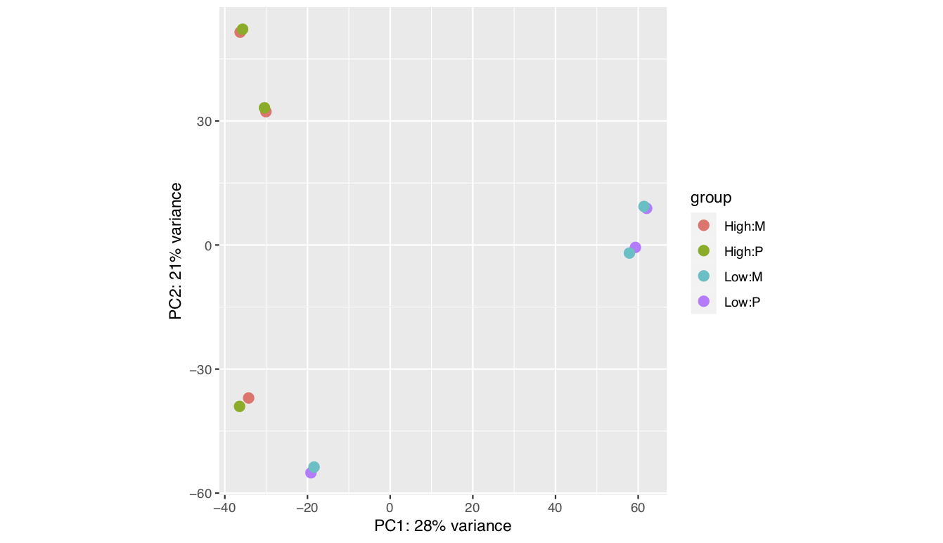
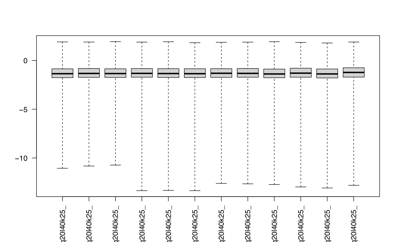
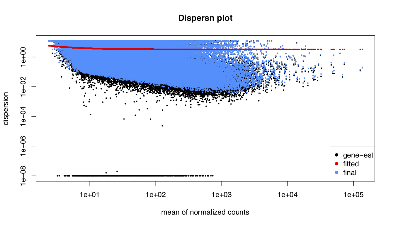
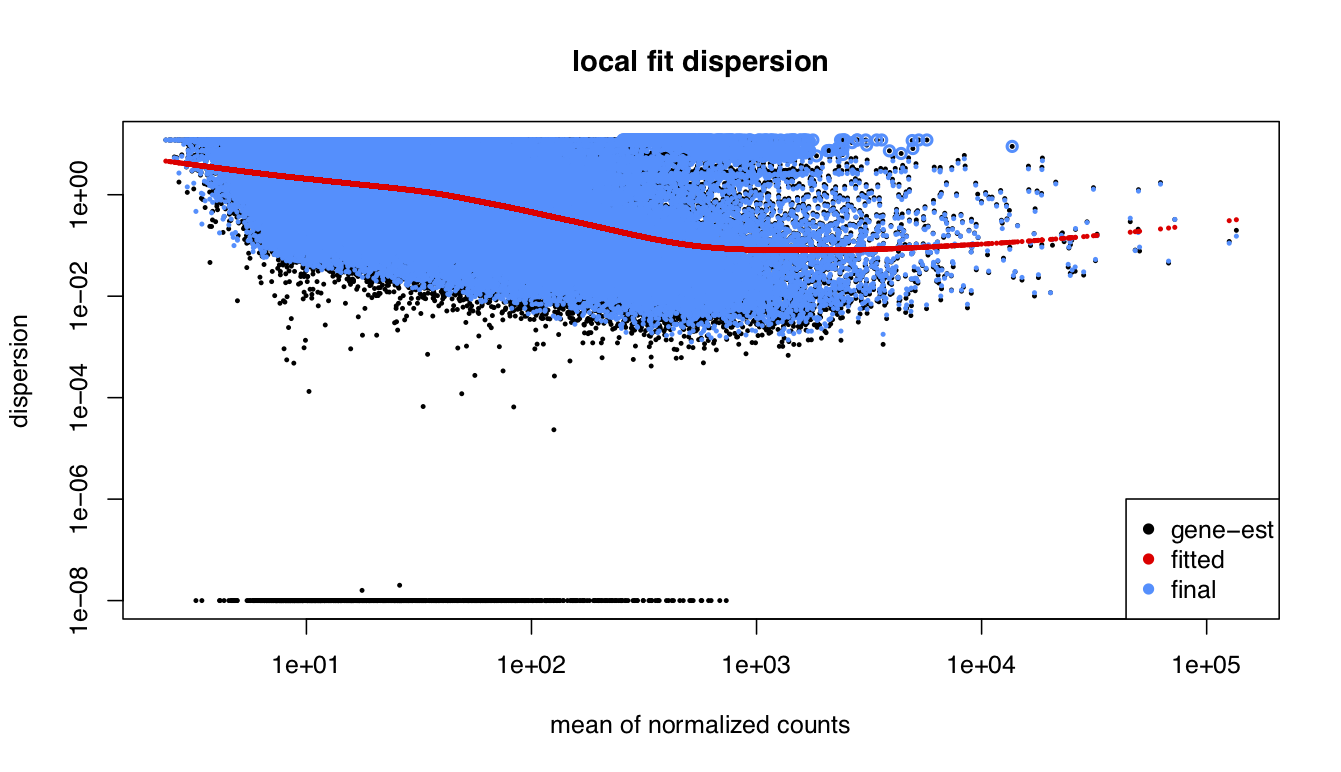
I been analysing some bulk rnaseq data of a non-model plant, looking at two treatments and two tissue stages. We used transcripts and salmon counts for looking at DEGs. Looking through the pca, cooks and dispersion plot (see below) – I been wondering if there is a concern of potential outlier samples/high variance as I notice one sample from each stage is away from the other two samples. The biological replicates are from three different trees – so there will be an element of biological variance due to that. So to account for that I have tried to fit two surrogate variables using sva (Note: I have also filtered some of the low count samples). Another concern was the dispersion plot – noticed the fitted line was one but this improves when a ‘local fit’ has been carried out. So I been wondering if it’s safe to go ahead and analyse the DEGs as is and potential bias I may be carrying forward. So was wondering if anyone could advice on this. Any thoughts would be much appreciated. Thanks in advance

#Create deseq object and run deseq
ddsTxi <- DESeqDataSetFromTximport(txi,colData = samples, design = ~ trt + Tissue)
ddsTxi
dds <- DESeq(ddsTxi)
#check data with plots
vsd <- vst(dds,blind=FALSE)
plotPCA(vsd,intgroup=c("trt","Tissue"))
#look at cooks distances
cooks <- log10(assays(dds)[["cooks"]])
boxplot(cooks, range=0, las=2)
nrow(dds)
keep <- rowSums(counts(dds) >= 10) >= 3 #at least3 samples with a count of 10 or higher
dds_filt <- dds[keep,]
dds_filt_loc <- estimateDispersions(dds_filt, fitType = "local")
nrow(dds_filt)
#percentage removed
nrow(dds_filt)/ nrow(dds)
vsd <- vst(dds_filt,blind=FALSE)
plotPCA(vsd,intgroup=c("trt","Tissue"))
#Disperssion plot on collapsed data
plotDispEsts(dds_filt, main="Dispersn plot")
plotDispEsts(dds_filt_loc,main="local fit dispersion")

#SVA
dat  <- counts(dds_filt, normalized = TRUE)
idx  <- rowMeans(dat) > 1
dat  <- dat[idx, ]
mod  <- model.matrix(~ trt + Tissue, colData(dds_filt))
mod0 <- model.matrix(~   1, colData(dds_filt))
svseq <- svaseq(dat, mod, mod0, n.sv = 2)
svseq$sv

par(mfrow = c(2, 1), mar = c(3,5,3,1))
for (i in 1:2) {
  stripchart(svseq$sv[, i] ~ dds_filt$trt, vertical = TRUE, main = paste0("SV", i))
  abline(h = 0)
 }

Sorry, for some reason I missed this post last week.

"The biological replicates are from three different trees"

Do you have the information about the tree? Are the three trees driving the three groups in the PCA plot above? If you have the tree information, you should include in the design as a covariate.