
Hi all,
I am trying to analyze 43 RRBS samples using edgeR and I am having some issues as I am very new to this. I mainly follow section 4.7 of the manual (https://www.bioconductor.org/packages/release/bioc/vignettes/edgeR/inst/doc/edgeRUsersGuide.pdf) to perform my analysis.
My DGEList obj looks like that:
>iclock_filtered
An object of class "DGEList"
$counts
            S_898-Me S_898-Un S_897-Me S_897-Un S_899-Me S_899-Un S_900-Me S_900-Un S_901-Me S_901-Un S_902-Me S_902-Un S_903-Me S_903-Un S_904-Me S_904-Un S_905-Me S_905-Un
chr1-567240        1       12        0       20       13      100        2       42       16       64        3       44        4       73        5       61        4        7
chr1-763078        0       26        0       19        1       18        0       10        0       10        0       13        0        6        0       10        0       13
chr1-763080        0       26        0       19        0       20        0        9        0        8        0        7        0        6        0        7        0       13
chr1-763088        1       25        0       19        0       20        0       10        0       10        0       13        0        6        0       10        1       12
chr1-763091        1       25        0       19        0       20        0       10        0       10        0       13        0        6        0       10        1       12
            S_906-Me S_906-Un S_907-Me S_907-Un S_908-Me S_908-Un S_909-Me S_909-Un S_911-Me S_911-Un S_912-Me S_912-Un S_913-Me S_913-Un S_914-Me S_914-Un S_915-Me S_915-Un
chr1-567240        3       27        3       18        3       48       10      121        2       18        0       21        8       50        0       16        9       31
chr1-763078        0       12        0        6        1       28        0       13        0       15        0        9        2        7        0       12        1       15
chr1-763080        0       10        0        6        0       21        0       13        0       15        0        6        0        9        0        9        1       15
chr1-763088        0       12        1        5        0       29        0       13        0       15        0        9        0        9        0       12        1       15
chr1-763091        1       11        0        6        0       29        0       13        0       15        0        9        0        9        0       12        0       16
3013 more rows ...

$samples
           group lib.size norm.factors
S_898-Me batch_2   328726            1
S_898-Un batch_2   328726            1
S_897-Me batch_2   308878            1
S_897-Un batch_2   308878            1
S_899-Me batch_2   452270            1
81 more rows ...

$genes
             Chr  Locus  EntrezID       Symbol Strand Distance Width
chr1-567240 chr1 567240 101928626 LOC101928626      -   -61769  1630
chr1-763078 chr1 763078 100288069 LOC100288069      -   -15556 52876
chr1-763080 chr1 763080 100288069 LOC100288069      -   -15554 52876
chr1-763088 chr1 763088 100288069 LOC100288069      -   -15546 52876
chr1-763091 chr1 763091 100288069 LOC100288069      -   -15543 52876
3013 more rows ...
And I also have a matadata table that looks like that:
>metadata
       ID   Batch Batch_Color Annotation Annotation_color gender                                                                File
1   S_898 batch_2           2       case                1      2  E:/pMedGR/analysis/input_files/CpG_context_00898_S2.bismark.cov.gz
2   S_897 batch_2           2       case                1      1  E:/pMedGR/analysis/input_files/CpG_context_00897_S1.bismark.cov.gz
3   S_899 batch_2           2       case                1      2  E:/pMedGR/analysis/input_files/CpG_context_00899_S3.bismark.cov.gz
4   S_900 batch_2           2       case                1      2  E:/pMedGR/analysis/input_files/CpG_context_00900_S4.bismark.cov.gz
5   S_901 batch_2           2       case                1      1  E:/pMedGR/analysis/input_files/CpG_context_00901_S5.bismark.cov.gz
6   S_902 batch_3           3       case                1      1  E:/pMedGR/analysis/input_files/CpG_context_00902_S6.bismark.cov.gz
7   S_903 batch_3           3       case                1      2  E:/pMedGR/analysis/input_files/CpG_context_00903_S1.bismark.cov.gz
8   S_904 batch_3           3       case                1      2  E:/pMedGR/analysis/input_files/CpG_context_00904_S2.bismark.cov.gz
9   S_905 batch_3           3       case                1      1  E:/pMedGR/analysis/input_files/CpG_context_00905_S3.bismark.cov.gz
10  S_906 batch_3           3       case                1      1  E:/pMedGR/analysis/input_files/CpG_context_00906_S4.bismark.cov.gz
11  S_907 batch_3           3       case                1      2  E:/pMedGR/analysis/input_files/CpG_context_00907_S5.bismark.cov.gz
12  S_908 batch_3           3       case                1      2  E:/pMedGR/analysis/input_files/CpG_context_00908_S6.bismark.cov.gz
13  S_909 batch_3           3    control                2      1  E:/pMedGR/analysis/input_files/CpG_context_00909_S7.bismark.cov.gz
14  S_911 batch_3           3    control                2      2  E:/pMedGR/analysis/input_files/CpG_context_00911_S9.bismark.cov.gz
15  S_912 batch_3           3    control                2      2 E:/pMedGR/analysis/input_files/CpG_context_00912_S10.bismark.cov.gz
16  S_913 batch_2           2    control                2      1 E:/pMedGR/analysis/input_files/CpG_context_00913_S11.bismark.cov.gz
17  S_914 batch_3           3    control                2      1 E:/pMedGR/analysis/input_files/CpG_context_00914_S12.bismark.cov.gz
18  S_915 batch_2           2    control                2      1  E:/pMedGR/analysis/input_files/CpG_context_00915_S7.bismark.cov.gz
19  S_917 batch_2           2    control                2      2  E:/pMedGR/analysis/input_files/CpG_context_00917_S8.bismark.cov.gz
20  S_918 batch_2           2    control                2      1  E:/pMedGR/analysis/input_files/CpG_context_00918_S9.bismark.cov.gz
21  S_920 batch_2           2    control                2      1 E:/pMedGR/analysis/input_files/CpG_context_00920_S10.bismark.cov.gz
22 S_1450 batch_4           4       case                1      2  E:/pMedGR/analysis/input_files/CpG_context_01450_S2.bismark.cov.gz
My goal is to find the regions that are differentially methylated between case and control samples Executing the model.matrix function as it is suggested in the manual I get the following:
>designSL <- model.matrix(~0+Annotation, data=metadata)
>designSL
   Annotationcase Annotationcontrol
1               1                 0
2               1                 0
3               1                 0
4               1                 0
5               1                 0
6               1                 0
7               1                 0
8               1                 0
9               1                 0
10              1                 0
11              1                 0
12              1                 0
13              0                 1
14              0                 1
15              0                 1
16              0                 1
17              0                 1
18              0                 1
19              0                 1
20              0                 1
21              0                 1
22              1                 0
23              1                 0
24              1                 0
25              1                 0
26              1                 0
27              0                 1
28              0                 1
29              0                 1
30              0                 1
31              0                 1
32              0                 1
33              1                 0
34              1                 0
35              0                 1
36              1                 0
37              0                 1
38              1                 0
39              1                 0
40              0                 1
41              0                 1
42              0                 1
43              0                 1
attr(,"assign")
[1] 1 1
attr(,"contrasts")
attr(,"contrasts")$Annotation
[1] "contr.treatment"
I then execute design <- modelMatrixMeth(~designSL) and I try to calculate the dispersion to get the following error:
> y1 <- estimateDisp(iclock_filtered, design=design)
Error in glmFit.default(sely, design, offset = seloffset, dispersion = 0.05,  :
  Design matrix not of full rank.  The following coefficients not estimable:
 designSLAnnotationcontrol
Reading other posts I suspect that I have to drop designSLAnnotationcontrol column from my design, but I am not sure I understand why I have to do this and what I am doing wrong.
I would appreciate any help to understand this.
Thank you in advance Leonardos

Dear Dr Smyth,
Thank you very much for your time and help. I am trying to wrap my head around this type of analysis and your comments are very useful. Indeed removing the ~ worked but I would like to ask some additional questions before I proceed to differential methylation analysis.
From section 3.7.3 I understand that I should not apply TMM normalization for this type of data. Setting the library sizes to be equal for each pair of libraries is enough. Is my understanding correct?
Based on your suggestions I now changed my code to include the following confounding factors:
As you can see I include age which is a continuous variable. Is that ok?
Is this plot ok to proceed with my analysis? Is there a section on your documentation that can explain this plot to a biologist?
Once again thank you very much for your time and help.
Best
Leonardos
You need to follow the edgeR case study closely.
The case study says that no other normalization is necessary. It says "Other normalization methods developed for RNA-seq data are not required for BS-seq data".
The case study uses
trend=FALSEforestimateDisp.There is no particular problem with the BCV plot except that variability in your experiment is high. The meaning of BCV is explained in Section 2.9 of the User's Guide.
Dear Dr Smyth
Thank you once again for your help. As I am very new to this |I am trying to understand why I have to do things like the case study. For example it is still not crystal clear for me why we dont need any other normalization or why we need the trend="none" argument in the dispersion calculation.
Either way I added trend=FALSE and after that I tried to identify differentialy expressed regions based on my case and control groups (using as confounding factors Batch, Age and Gender) adding the following bits:
fit <- glmFit(y, design)
lrt <- glmLRT(fit)
Is that the correct way or do I need to use the contrast or coef arguments somehow? Doing the analysis like that returns 0 significant results and I am not sure if I am doing something wrong. Just to be clear the last columns of my design matrix looks like so: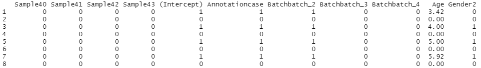
Thank you very much once again.
Yes, you need to set
coef = "Annotationcase".How else would edgeR know which variable you want to test for?
Dear Dr Smyth,
Everything makes much more sense now although I still dont get any significant results. Can this be due to the low number of samples (22 cases vs 21 controls)?
If I want to look for differentially expressed regions with respect to age (a continuous variable), controlling for batch and phenotype I can just change my model to designSL <- model.matrix(~Age+Batch+Annotation) and then do lrt <- glmLRT(fit, coef="Age")? Does it matter that age is not discrete?
Once again thank you very much for your time.
Yes, it works the same for any variable. It does not matter than Age is continuous.
Dear Dr Smyth,
Thx a lot for explaining all that to me.
Reading the manual and some posts I understand that glmQLFit sometimes behaves better than glmFit. Is that applicable for my analysis as well?
For methylation data, please stick to glmFit() and glmLRT(), same as in the case study in the User's Guide. Using glmQLFit would not give more DE results.
Dear Dr Smyth,
I am trying to understand why my analysis has no significant results and I noticed that in the example in the manual you are using designSL <- model.matrix(~0+Group, data=targets). In my analysis I do not include the 0+ bit.
If I add this bit to my model and change my code to that: designSL <- model.matrix(~0+Annotation+Batch + Age + Gender) and keeping everything else the same gives me some significant hits.
I am not sure if this is correct though. Can you explain the differences of having 0+ in the formula? Should I stick to the example and keep the 0+?
Thx a lot once again for your time and help. Best Leonardos
No, it is quite wrong to change the design matrix while keeping all other code the same.
There is no reason for using
0+when you only have two groups. There is lots of documentation on how to form design matrices and how to use0+, in the edgeR User's Guide as well as other places.