Hi,

I am interested in fitting gene expression in two different stages of development (RNA-seq counts, quantile-normalised, and log1p-transformed). Based on visualising a scatter plot of the two stages, I have noticed that variance is not as high for higher levels of gene expression, compared for genes with lower values of gene expression. I have learned this is called heteroscedasticity and I would like to account for it in order to model properly.

hco <- hcor_ab[[1]] # this is a data frame with two columns 'a' and 'b' corresponding to two stages, and 3641 rows corresponding to genes

jsd_value <- 0 # a value that I need in the plot below

hco_lm <- lm(b ~ a, data = hco)

library(ggpointdensity)
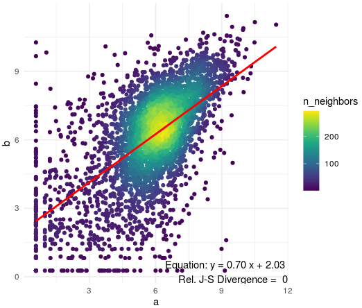
  ggplot(data = hco,mapping = aes(x=a,y=b)) +
    labs(title = names(hcor_ab)[1] ) +
    geom_pointdensity()+
    stat_smooth(method = "lm", se = FALSE, color = "red") + 
    theme_minimal()+
    scale_color_viridis()+
    annotate(
      "text", x = Inf, y = -Inf, hjust = 1, vjust = 0, 
      label = paste(
        "Equation: y =", sprintf("%.2f", coef(summary(lm(b ~ a, data = hco)))[2, 1]), "x +", 
        sprintf("%.2f", coef(summary(lm(b ~ a, data = hco)))[1, 1]), "\n",
        "Rel. J-S Divergence = ", jsd_value
        )
      )

See below the resulting plot of this code.

To account for heteroscedasticity, I have been advised to use the inverse of the expected sampling variance as weights, and to compute bootstraps for this. But I am at a loss on how to proceed.

One extra thing to consider: I have to implement this inside a larger function that takes the two-condition data frame as input, to be run by other end-users, so in principle it would be in my best interest to rely just on the data that is fed to the function (the hco object) and no other a-priori information.

Thank you very much in advance!

One thing you can do, especially helpful if you are working with arbitrary transformations, is to compute the bootstrap variance of the data after transformation. This is pretty easy to do with tximport/tximeta, if you have computed bootstraps. Read: you will have had to run kallisto or Salmon while specifying a number of bootstraps. We often use 20-30 bootstraps.

Try this:

txi <- tximport(files, ...)
inf_reps <- txi$infReps
transformed_inf_reps <- lapply(inf_reps, transformation)
vars <- sapply(transformed_inf_reps, rowVars)