I got the network with the WGCNA package and then imported the network into Cytoscape. I applied the analyzer network to obtain the "degree" (I assume that this is the degree of connectivity that will allow me to choose the hub genes.) but the results seem strange to me and I don't know where the error could be, could you please give me some guidance in this regard? Thank you very much in advance

Code should be placed in three backticks as shown below

# R studio V 4.2.3
#loading data
datExpr <- read.csv("TPM_Zscore_Ready.csv", header=TRUE,  sep=',')
colnames(datExpr)

# Manipulate file so it matches the format WGCNA needs
row.names(datExpr) = datExpr$Genes
datExpr$Genes = NULL
datExpr = as.data.frame(t(datExpr)) # now samples are rows and genes are columns
dim(datExpr) 

# detect outlier genes
gsg = goodSamplesGenes(datExpr, verbose = 3)
gsg$allOK 
summary(gsg)

## If the last statement returns TRUE, all genes have passed the cuts. If not, is removed the offending genes and samples from the data.
#datExpr <- datExpr[gsg$goodGenes == TRUE,] 

####### Uploading the Trait file ################
#Create an object called "datTraits" that contains your trait data
datTraits = read.csv("Traits_ready.csv") 

#form a data frame analogous to expression data that will hold the traits.
rownames(datTraits) = datTraits$Sample
datTraits$Sample = NULL
table(rownames(datTraits)==rownames(datExpr)) 

# You have finished uploading and formatting expression and trait data
# Expression data is in datExpr, and the corresponding traits are in datTraits
datTraits<-datTraits #[,-1]

##########clustering data and traits
#  Calculate sample distance and cluster the samples 
# cluster samples
sampleTree2 <- hclust(dist(datExpr), method = "average")

# Convert traits to a color representation: white means low, red means high, grey means missing entry
traitColors <- numbers2colors(datTraits, signed = FALSE)

# Choosing a soft-threshold to fit a scale-free topology to the network
# Call the network topology analysis function
powers = c(c(1:10), seq(from =12, to=50, by=2)) 

sft = pickSoftThreshold(datExpr,
                        dataIsExpr = TRUE,
                        powerVector = powers,
                        corFnc = cor,                             
                        corOptions = list(use = 'p'), 
                        verbose = 5,                              
                        networkType = "signed")                           

sft.data <-sft$fitIndices
write.table(sft, file = "sft_result.txt", sep = ",", quote = FALSE, row.names = T)

#  Turn data expression into topological overlap matrix (TOM)
softPower = 40

# Generating adjacency and TOM diss/similarity matrices based on the selected soft-power"
#Calculation of the topological overlap matrix, and the corresponding dissimilarity, from a given adjacency matrix.
adjacency <- adjacency(datExpr, type = "signed", power = softPower)
TOMadj <- TOMsimilarity(adjacency)
dissTOM <- 1- TOMadj
dim(dissTOM)
#save(dissTOM, softPower, file="table_DissTOM.RData") 
#load("table_DissTOM.RData")

#  Construct modules by Clustering using TOM
# Call the hierarchical clustering function. There is used the pearson correlation (average)
hclustGeneTree <- hclust(as.dist(dissTOM), method = "average")

# Make the modules larger, so set the minimum higher
minModuleSize <- 30

# Module ID using dynamic tree cut
dynamicMods <- cutreeDynamic(dendro = hclustGeneTree, 
                             distM = dissTOM,
                             deepSplit = 2, pamRespectsDendro = FALSE,
                             minClusterSize = minModuleSize)
table(dynamicMods)
length(table(dynamicMods))

# Convert numeric labels into colors
dynamicColors = labels2colors(dynamicMods)      
#sort(table(dynamicColors), decreasing = TRUE)   # get the number of genes by color
table(dynamicColors)

#  Merge modules
# Calculate eigengenes
dynamic_MEList <- moduleEigengenes(datExpr, colors = dynamicColors)
dynamic_MEs <- dynamic_MEList$eigengenes
# Calculate dissimilarity of module eigengenes
dynamic_MEDiss <- 1-cor(dynamic_MEs)
# Cluster module eigengenes
dynamic_METree <- hclust(as.dist(dynamic_MEDiss), method = "average")
# Plot the hclust
sizeGrWindow(7,6)
plot(dynamic_METree, main = "Dynamic Clustering of module eigengenes",
     xlab = "", sub = "")

# Merge close modules
### height cut of 0.2, corresponding to correlation of 0.80, to merge module with 90% of similarity
dynamic_MEDissThres <- 0.2 
# Plot the cut line
abline(h = dynamic_MEDissThres, col = "red")

# Call an automatic merging function
merge_dynamic_MEDs <- mergeCloseModules(datExpr, dynamicColors, cutHeight = dynamic_MEDissThres, verbose = 3)
# The Merged Colors
dynamic_mergedColors <- merge_dynamic_MEDs$colors

# Eigen genes of the new merged modules
mergedMEs <- merge_dynamic_MEDs$newMEs
mergedMEs

write.table(merge_dynamic_MEDs$oldMEs,file="oldMEs.txt")
write.table(merge_dynamic_MEDs$newMEs,file="newMEs.txt")


#===============================================================================
#  Export of networks (for me only new MEs) to external software (Cytoscape)
#===============================================================================


for (i in 1:length(merge_dynamic_MEDs$newMEs)){
  modules = c(substring(names(merge_dynamic_MEDs$newMEs)[i], 3));
  genes = colnames(datExpr)
  inModule = is.finite(match(dynamic_mergedColors,modules)) 
  modGenes = genes[inModule]
  modTOM=dissTOM[inModule,inModule]
  dimnames(modTOM)=list(modGenes,modGenes)
  cyt = exportNetworkToCytoscape(modTOM,
                                 edgeFile = paste("output_for_cytoscape/merge_CytoscapeInput-edges-", paste(modules, collapse="-"), ".txt", sep=""),
                                 nodeFile = paste("output_for_cytoscape/merge_CytoscapeInput-nodes-", paste(modules, collapse="-"), ".txt", sep=""),
                                 weighted = TRUE, threshold = -1, nodeNames = modGenes, nodeAttr = dynamicColors[inModule]);
}

#===============================================================================
#  Networks to Cytoscape
#===============================================================================

library(RCy3)
cytoscapePing () # make sure cytoscape is open
cytoscapeVersionInfo ()
# cytoscapeVersion "3.10.0" 

#### Module white 

# use the connection with Cytoscape through the 'RCy3' package
#loading file from cyt
edge <- read.delim("merge_CytoscapeInput-edges-white.txt")
colnames(edge)
# it need to modify colnames
colnames(edge) <- c("source", "target", "weight", "direction","fromAltName", "toAltName")

node <- read.delim("merge_CytoscapeInput-nodes-white.txt")
colnames(node)
# it need to modify colnames
colnames(node) <- c("id" , "altName", "node_attributes")

createNetworkFromDataFrames(node,edge, title="white network", collection="DataFrame white")
#createNetworkFromDataFrames(node,edge[1:50,], title="white network", collection="DataFrame white")

#use other pre-set visual style
setVisualStyle('Marquee')

# set up my own style
style.name = "myStyle"
defaults <- list(NODE_SHAPE="ellipse",
                 NODE_SIZE=30,
                 EDGE_TRANSPARENCY=120,
                 NODE_LABEL_POSITION="W,E,c,0.00,0.00")
nodeLabels <- mapVisualProperty('node label','id','p')
nodeFills <- mapVisualProperty('node fill color','node_attributes','d',c("A","B"), c("#FF9900","#66AAAA"))
arrowShapes <- mapVisualProperty('Edge Target Arrow Shape','interaction','d',c("activates","inhibits","interacts"),c("Arrow","T","None"))
edgeWidth <- mapVisualProperty('edge width','weight','p')

createVisualStyle(style.name, defaults, list(nodeLabels,nodeFills,arrowShapes,edgeWidth))
setVisualStyle(style.name)

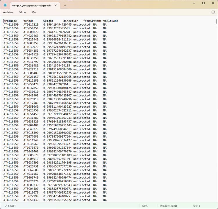
Edges

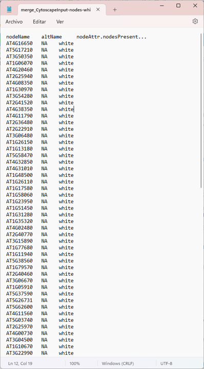
nodes

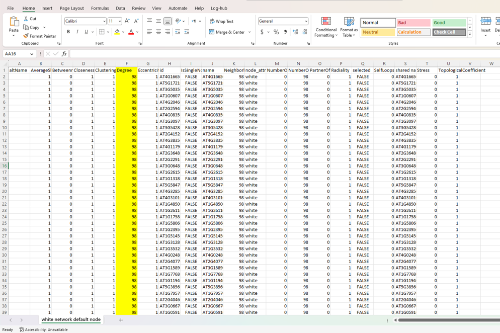
Results from analyzer network

Hi. I can't fully reproduce this case without the starting input files. Even better would be the node and edge files, since those are all I need to reproduce the RCy3-relevant steps:

• merge_CytoscapeInput-edges-white.txt
• merge_CytoscapeInput-nodes-white.txt

A screenshot of the network in Cytoscape might also be sufficient as my initial guess is that you are calculating values between all pairs of nodes. This would produce a networks where each node is connected to all other nodes. If there are 99 nodes, then the degree would be 98 for every node, which is exactly what you are seeing.

I suspect what you want to do is to delete edges based on the weight attribute. Then you would have a more interesting network topology to work with. It would have a distribution of degrees and you could then identify hubs, etc.