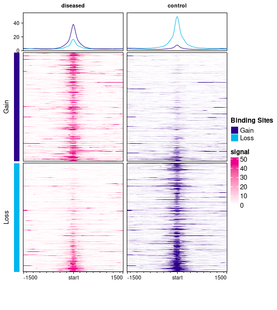
This plot has two columns, one for diseased (plotted in magenta) and one for control (plotted in purple) samples. There are two sets of peaks: Gain peaks (higher in diseased), represented by dark blue, and Loss peaks (higher in control), represented in cyan.
Each column has three plots showing the signal (read density) in windows centered on each binding site and expanding 1500bp up- and down-stream. By default, the read density is computed by taking the average normalized read counts across all the samples in each sample group (diseased and control).
The top plots each contain curves showing the mean read density over all the samples in each group across all the binding sites; there is a curve for signal across the Gain sites (dark blue curve) and for the Loss sites (cyan curve). In the first column (diseased), the dark blue curve is higher than the cyan curve, indicating the higher binding levels in diseased samples, while in the second (control) column, the cyan (Loss) sites show higher signal (with the degree of Loss in the second column being greater than the degree of Gain in the first column).
The remaining two plots in each column show the read density for windows around each binding site. The top plots show signal in and around Gain binding sites (averaged across the samples in the diseased group on the left, in magenta, and the control samples on the right, in purple). The signal is higher in the diseased samples (as expected for Gain sites). The bottom plots show mean read count levels in windows in and around the Loss binding sites (with a greater signal in the right-hand control sites).
The help page for dba.plotProfile() offer some more details, as does a workbook available here:
https://content.cruk.cam.ac.uk/bioinformatics/software/DiffBind/plotProfileDemo.html


Thanks Rory! So that means the diseased sample has chromatin more open then the control one, is that correct?
Not necessarily. It look to me like there is reconfiguring going on, with some chromatin that was open in the control becoming closed (the Loss regions) and others becoming more open (the Gain sites). You can compare how many sites were Gain vs Lost to see if it is opening more in one condition or the other. An MA plot (
dba.plotMA()) is probably a better way to see this balance.Thank you for the explanation! The purple (gain) in the control in the right bottom corner but on the y axis is labeled loss which I am confused. Would you please explain a bit? So gain mean more open and loss mean close and the magenta signal value higher mean more open, is that correct?
I can see the confusion here as one color is being used in two different ways.
The dark blue/purple color is used for the bars on the left-hand side, and in the curves in the top row, to represent Gain sites (great binding in disease). Within the main heatmaps, the two colors (magenta and purple) are used to represent the two sample groups. So signal in the disease samples are drawn using a magenta color scale, while signal in the control sample is drawn using a purple color scale. This use of purple is separate from its use in the curve plots at the top. I'll have a look at altering the default colors to avoid this confusion.
In the meantime, you can change the colors used for the heat map to make things more clear:
where the disease sample group will be plotted on a magenta scale and the control group will be plotted on a dark green scale.
Hi Rory, when I run your code, I got this error:
If I run:
Error: unexpected ',' in "dba.plotProfile <- (profiles,"
Would you have a look? Thank you so much!
Hi Rory. There are so many red dot above and below the blue line so it is hard to know which condition are more open, is that correct? Is 115941 sites are too high which I did something wrong?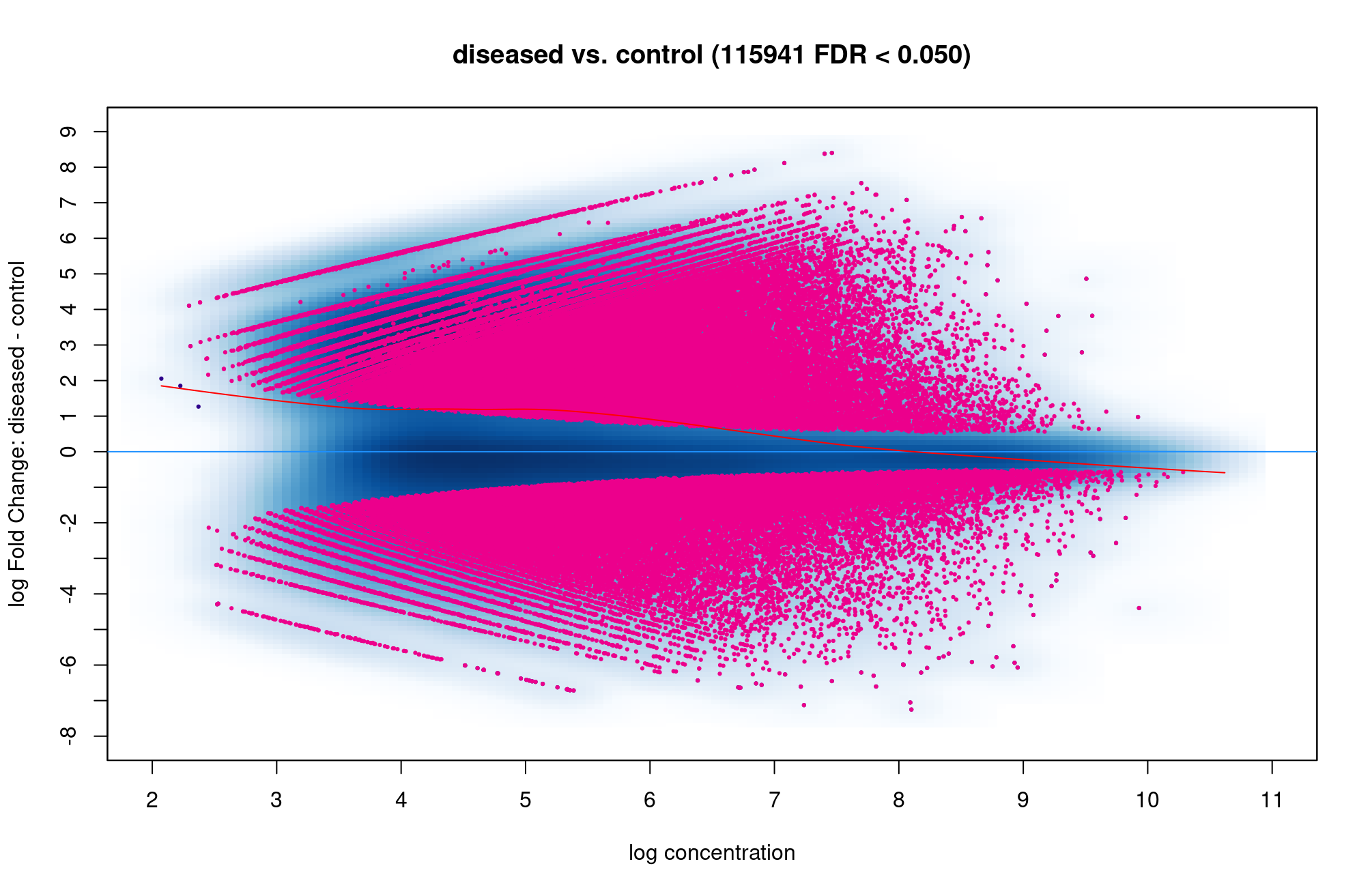
That does seem like you have a very high number of open chromatin sites changing. How many are in the consensus matrix?
You can see how many are opening in the disease state vs closing by subsetting the
dba.report():Thank you so much. I think the function is
dba.report(). more_open_in_disease: 79113 more_closed_in_disease: 36828 So there are 79113 peaks that are more open in disease than in control, is that correct? Hope that value is not unusual.If I want to find genes that are more open in diseased than control, I can filter out peaks that have highest log2Fold change like this, is that correct?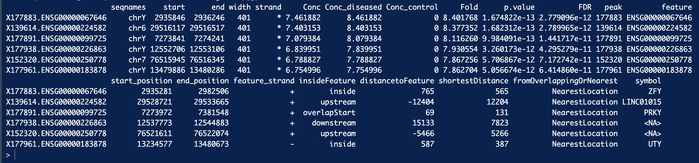 Thank you!
See above, you want the sites where
Fold > 0.I sorted Fold decreasing. When I filter out genes with fold > 2.5 and filter out genes with fold < -2.5 and got 1287 genes appear in both side. Is that possible? Thank you so much :smiley:
It is possible but unlikely that you'd get the exact same number of genes gaining and losing binding levels, maybe check your code?
Also, when you filter on fold change, this actually changes the null hypothesis your are using for the statistical test. You should instead set the
foldparameter when callingdba.report()which will re-compute the FDR appropriately, as you are now testing for sites who's binding affinity changes by at least 2.5 fold.Finally, the fold is specified as a log2 value, so if you are filtering on
$Fold > 2.5you should use$Fold > log2(2.5).