
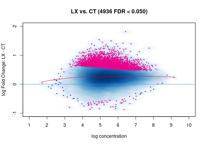
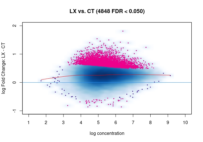
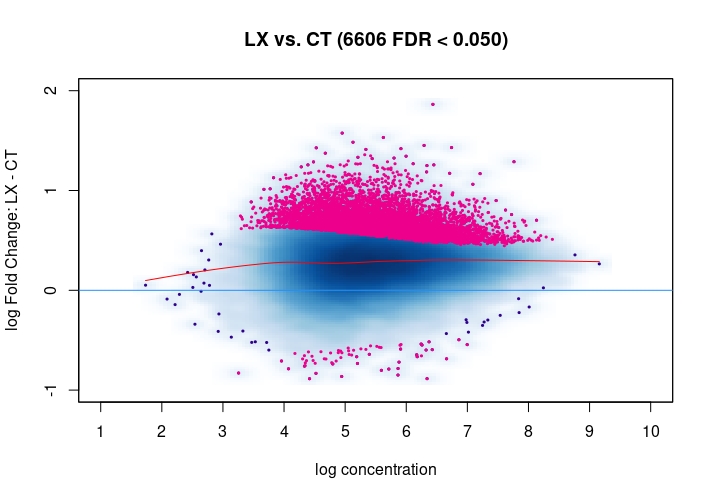
Hi, I have been using DiffBind_3.0.7 for determining Differential accessible sites. I have CT and KD samples, 3 replicates each, and we expect a large scale opening of the chromatin in the KD. After calling Peaks with MACS2 and running the DiffBind steps, I used 3 different Normalization commands to see how or whether they differ significantly in terms of numbers of differentially open sites . I read the Normalization part of your Vignette, and it mentions that one of the recommendations for atac-seq is actually the second option I use. I was wondering if the first option would be a valid way. Also, a full library size normalization ( option 3 ) should be similar to option 2, but I get much more sites. Would you recommend I stick with Option 2 ? I am attaching the MA plots ( Options 1,2 and 3 )
Also, if in a situation where I do no expect widespread changes of chromatin accessibility, would you recommend RLE on Reads in Peaks normalization?
Thank you, Debayan
Code should be placed in three backticks as shown below
mod_atacseq_data.norm1 <- dba.normalize(mod_atacseq_data, method=DBA_DESEQ2, normalize=DBA_NORM_LIB, library=DBA_LIBSIZE_BACKGROUND, background=TRUE)
mod_atacseq_data.norm2 <- dba.normalize(mod_atacseq_data, method=DBA_DESEQ2, normalize=DBA_NORM_NATIVE, library=DBA_LIBSIZE_BACKGROUND, background=TRUE)
mod_atacseq_data.norm3 <- dba.normalize(mod_atacseq_data, method=DBA_DESEQ2, normalize=DBA_NORM_LIB, library=DBA_LIBSIZE_FULL, background=FALSE)

#Contrasts#
mod_atacseq_data.norm1.ctst <- dba.contrast(mod_atacseq_data.norm1, minMembers=3, categories=DBA_CONDITION)
mod_atacseq_data.norm2.ctst <- dba.contrast(mod_atacseq_data.norm2, minMembers=3, categories=DBA_CONDITION)
mod_atacseq_data.norm3.ctst <- dba.contrast(mod_atacseq_data.norm3, minMembers=3, categories=DBA_CONDITION)

#Differential Analysis#
mod_atacseq_data.results1 <- dba.analyze(mod_atacseq_data.norm1.ctst, method=DBA_DESEQ2)
mod_atacseq_data.results2 <- dba.analyze(mod_atacseq_data.norm2.ctst, method=DBA_DESEQ2)
mod_atacseq_data.results3 <- dba.analyze(mod_atacseq_data.norm3.ctst, method=DBA_DESEQ2)

mod_atacseq_data.DB1 <- dba.report(mod_atacseq_data.results1, method=DBA_DESEQ2, bCalled=T, bCounts=T)
mod_atacseq_data.DB2 <- dba.report(mod_atacseq_data.results2, method=DBA_DESEQ2, bCalled=T, bCounts=T)
mod_atacseq_data.DB3 <- dba.report(mod_atacseq_data.results3, method=DBA_DESEQ2, bCalled=T, bCounts=T)

bindingdata1=as.data.frame(mod_atacseq_data.DB1)
bindingdata2=as.data.frame(mod_atacseq_data.DB2)
bindingdata3=as.data.frame(mod_atacseq_data.DB3)


 sum(bindingdata1$Fold>0)
4882
> sum(bindingdata1$Fold<0)
54

> sum(bindingdata2$Fold>0)
4806
> sum(bindingdata2$Fold<0)
42

> sum(bindingdata3$Fold>0)
6543
> sum(bindingdata3$Fold<0)
63

dba.plotMA(mod_atacseq_data.results1)

dba.plotMA(mod_atacseq_data.results2)

dba.plotMA(mod_atacseq_data.results3)


sessionInfo( )
R version 4.0.2 (2020-06-22)
Platform: x86_64-pc-linux-gnu (64-bit)
Running under: CentOS Linux 7 (Core)

Matrix products: default
BLAS/LAPACK: /usr/lib64/libopenblasp-r0.3.3.so

locale:
 [1] LC_CTYPE=en_US.UTF-8       LC_NUMERIC=C               LC_TIME=en_US.UTF-8        LC_COLLATE=en_US.UTF-8
 [5] LC_MONETARY=en_US.UTF-8    LC_MESSAGES=en_US.UTF-8    LC_PAPER=en_US.UTF-8       LC_NAME=C
 [9] LC_ADDRESS=C               LC_TELEPHONE=C             LC_MEASUREMENT=en_US.UTF-8 LC_IDENTIFICATION=C

attached base packages:
[1] stats4    parallel  stats     graphics  grDevices utils     datasets  methods   base

other attached packages:
 [1] csaw_1.24.3                 DiffBind_3.0.7              SummarizedExperiment_1.20.0
 [4] MatrixGenerics_1.2.0        matrixStats_0.57.0          Hmisc_4.4-2
 [7] Formula_1.2-4               survival_3.1-12             lattice_0.20-41
[10] impute_1.64.0               EnsDb.Hsapiens.v79_2.99.0   ensembldb_2.14.0
[13] AnnotationFilter_1.14.0     GenomicFeatures_1.42.1      AnnotationDbi_1.52.0
[16] Biobase_2.50.0              GenomicRanges_1.42.0        GenomeInfoDb_1.26.1
[19] IRanges_2.24.0              S4Vectors_0.28.0            BiocGenerics_0.36.0
[22] forcats_0.5.0               purrr_0.3.4                 readr_1.4.0
[25] tidyr_1.1.2                 tidyverse_1.3.0             data.table_1.13.2
[28] stringr_1.4.0               dplyr_1.0.2                 ggfortify_0.4.11
[31] ggplot2_3.3.2               tibble_3.0.4                RColorBrewer_1.1-2
[34] pheatmap_1.0.12             readxl_1.3.1

loaded via a namespace (and not attached):
  [1] tidyselect_1.1.0         RSQLite_2.2.1            htmlwidgets_1.5.2        grid_4.0.2
  [5] BiocParallel_1.24.1      munsell_0.5.0            base64url_1.4            systemPipeR_1.24.2
  [9] withr_2.3.0              colorspace_2.0-0         Category_2.56.0          knitr_1.30
 [13] rstudioapi_0.13          bbmle_1.0.23.1           GenomeInfoDbData_1.2.4   mixsqp_0.3-43
 [17] hwriter_1.3.2            bit64_4.0.5              coda_0.19-4              batchtools_0.9.14
 [21] vctrs_0.3.5              generics_0.1.0           xfun_0.19                BiocFileCache_1.14.0
 [25] R6_2.5.0                 apeglm_1.12.0            invgamma_1.1             locfit_1.5-9.4
 [29] rsvg_2.1                 bitops_1.0-6             DelayedArray_0.16.0      assertthat_0.2.1
 [33] scales_1.1.1             nnet_7.3-14              gtable_0.3.0             rlang_0.4.9
 [37] genefilter_1.72.0        splines_4.0.2            rtracklayer_1.50.0       lazyeval_0.2.2
 [41] broom_0.7.2              brew_1.0-6               checkmate_2.0.0          BiocManager_1.30.10
 [45] yaml_2.2.1               modelr_0.1.8             backports_1.2.0          RBGL_1.66.0
 [49] tools_4.0.2              ellipsis_0.3.1           gplots_3.1.1             Rcpp_1.0.5
 [53] plyr_1.8.6               base64enc_0.1-3          progress_1.2.2           zlibbioc_1.36.0
 [57] RCurl_1.98-1.2           prettyunits_1.1.1        rpart_4.1-15             openssl_1.4.3
 [61] ashr_2.2-47              haven_2.3.1              ggrepel_0.8.2            cluster_2.1.0
 [65] fs_1.5.0                 magrittr_2.0.1           reprex_0.3.0             truncnorm_1.0-8
 [69] mvtnorm_1.1-1            SQUAREM_2020.5           amap_0.8-18              ProtGenerics_1.22.0
 [73] hms_0.5.3                xtable_1.8-4             XML_3.99-0.5             emdbook_1.3.12
 [77] jpeg_0.1-8.1             gridExtra_2.3            compiler_4.0.2           biomaRt_2.46.0
 [81] bdsmatrix_1.3-4          KernSmooth_2.23-17       V8_3.4.0                 crayon_1.3.4
 [85] htmltools_0.5.0          GOstats_2.56.0           geneplotter_1.68.0       lubridate_1.7.9.2
 [89] DBI_1.1.0                dbplyr_2.0.0             MASS_7.3-51.6            rappdirs_0.3.1
 [93] ShortRead_1.48.0         Matrix_1.2-18            cli_2.2.0                pkgconfig_2.0.3
 [97] GenomicAlignments_1.26.0 numDeriv_2016.8-1.1      foreign_0.8-80           xml2_1.3.2
[101] annotate_1.68.0          XVector_0.30.0           AnnotationForge_1.32.0   rvest_0.3.6
[105] VariantAnnotation_1.36.0 digest_0.6.27            graph_1.68.0             Biostrings_2.58.0
[109] cellranger_1.1.0         htmlTable_2.1.0          edgeR_3.32.0             GSEABase_1.52.0
[113] GreyListChIP_1.22.0      curl_4.3                 Rsamtools_2.6.0          gtools_3.8.2
[117] rjson_0.2.20             lifecycle_0.2.0          jsonlite_1.7.1           askpass_1.1
[121] limma_3.46.0             BSgenome_1.58.0          fansi_0.4.1              pillar_1.4.7
[125] httr_1.4.2               GO.db_3.12.1             glue_1.4.2               png_0.1-7
[129] bit_4.0.4                Rgraphviz_2.34.0         stringi_1.5.3            blob_1.2.1
[133] DESeq2_1.30.0            latticeExtra_0.6-29      caTools_1.18.0           memoise_1.1.0
[137] DOT_0.1                  irlba_2.3.3

Please show the MA-plots, you can use the image button to upload images (the one right of the
Codebutton).Sorry, I have just uploaded them. Thanks!
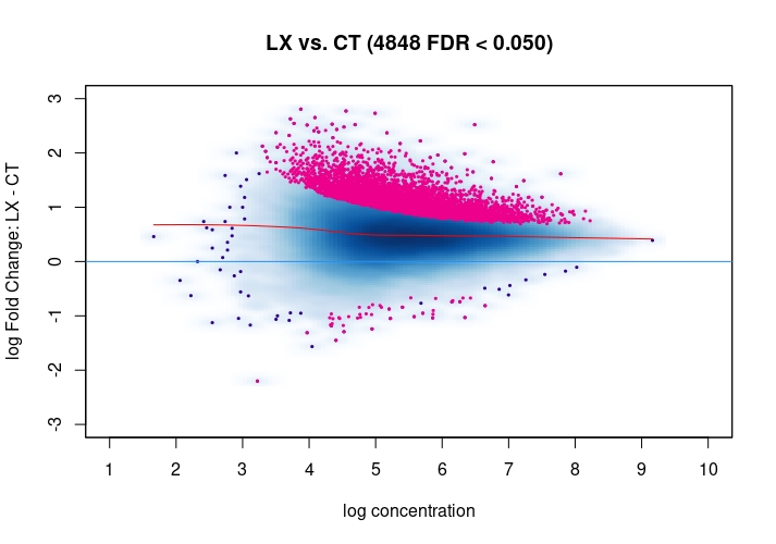
Just my two cents: Basically these plots look all the same. I would even argue that they are all offset towards the LX condition which is probably more of a normalization artifact than true biology. The data look kind of symmetric like in any other ATAC-seq experiment I've seen, supported by the local regression trend, and the fact that the bulk of the very high-count regions (far right) is also offset towards LX makes it even more questionable whether this is really true biology in terms of a general shift. I would strongly recommend to explore alternative normalization strategies and also check for confounders, e.g. FRiPs so whether data quality is notable different between data. See e.g. the
csawvignette for suggestions. I am not a DiffBind user so not sure what exactly the above strategies do, therefore suggestingcsawto explore data (edit:) as an independent approach.Also, it would be good to see the non-normalized MA plot!
Thanks a lot for your suggestion, I will try csaw as an independent approach. I have attached the non-normalized MA plot. There does appear to be deviation towards the y=0 line upon normalization, but as you mention there is a definite offset towards LX in the normalized MA plot