Question

DESeq2 anormally high estimation of Log2FoldChange

0

Entering edit mode

hugo.denis • 0

@user-24686

Last seen 3.1 years ago

Hello,

I am a new user of DESeq2 and I am having trouble with log2FoldChange calculation with latest version of DESeq2 package. DEGs reported in pairwise comparison using Wald Tests show completely abnormally high values of log2FoldChange (up to -30 and +20) I managed to recalculate an approximate of what would be a decent log2FoldChange per gene using

plotCounts

function and re-calculating log2foldChange for each gene as log2(mean(counts_condB))-log2(mean(counts_condA)). I know it is not exactly the way it is done in DESeq2 but I expect something close in term of order of magnitude. Values calculated this way where way lower and seemed to make more sense (at least there is no abs(log2FoldChange) above 10).

I can't really find what I am doing wrong here. I saw on a previous post that someone had a similar issue that was solved removing the parallel=T argument od DESeq function which I tried without sucess. You'll find below my code and infos.

dds<-DESeq2::DESeqDataSetFromMatrix(countData=sample_cts,colData=subset,design=~Mortalite+Temperature+Mortalite:Temperature+Batch+Manip)
keep<-rowSums(counts(dds) >= 10) >= 3
dds<-dds[keep,] 
dds$Mortalite <- relevel(dds$Mortalite, ref = "ok")
dds_Wald<-DESeq(dds,parallel=T,BPPARAM=MulticoreParam(30),test="Wald")
fullresnames<-resultsNames(dds_Wald)

res<-DESeq2::results(dds_Wald,name=fullresnames[2],alpha=0.01,lfcThreshold = 2)
head(data.frame(res) %>% subset(padj<0.01) %>% arrange(desc(abs(log2FoldChange))))

                       baseMean log2FoldChange    lfcSE      stat       pvalue         padj
TRINITY_DN10323_c0_g1_i1 11.97128            -30 4.869130 -5.750514 8.897229e-09 3.794748e-06
TRINITY_DN1044_c0_g1_i7  14.07173            -30 4.865994 -5.754220 8.704285e-09 3.794748e-06
TRINITY_DN2267_c2_g1_i12 18.34856            -30 4.863310 -5.757396 8.542143e-09 3.794748e-06
TRINITY_DN2356_c0_g1_i7  44.30817            -30 4.863334 -5.757367 8.543604e-09 3.794748e-06
TRINITY_DN2590_c0_g1_i5  29.76859            -30 4.863410 -5.757277 8.548156e-09 3.794748e-06
TRINITY_DN2614_c0_g1_i5  30.91978            -30 3.814330 -7.340740 2.124169e-13 2.687073e-10

plotCounts(dds_Wald, "TRINITY_DN10323_c0_g1_i1", intgroup="Mortalite")

enter image description here

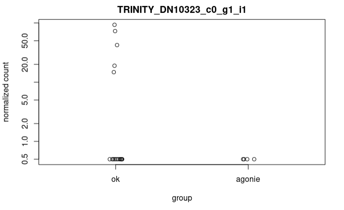
As you can see the log2FoldChange value is strange regarding the counts. If I calculate the log2FoldChange as described before :

x<-plotCounts(dds_Wald, "TRINITY_DN10323_c0_g1_i1" , intgroup="Mortalite",returnData = T) %>% group_by(Mortalite) %>% summarize(mean=mean(count))
log2(x$mean[x$Mortalite=="agonie"])-log2(x$mean[x$Mortalite=="ok"])
[1] -4.950851


sessionInfo()
R version 4.0.3 (2020-10-10)
Platform: x86_64-pc-linux-gnu (64-bit)
Running under: Ubuntu 20.04.2 LTS

Matrix products: default
BLAS:   /usr/lib/x86_64-linux-gnu/blas/libblas.so.3.9.0
LAPACK: /usr/lib/x86_64-linux-gnu/lapack/liblapack.so.3.9.0

Random number generation:
 RNG:     L'Ecuyer-CMRG 
 Normal:  Inversion 
 Sample:  Rejection 

locale:
 [1] LC_CTYPE=fr_FR.UTF-8       LC_NUMERIC=C               LC_TIME=fr_FR.UTF-8        LC_COLLATE=fr_FR.UTF-8     LC_MONETARY=fr_FR.UTF-8   
 [6] LC_MESSAGES=fr_FR.UTF-8    LC_PAPER=fr_FR.UTF-8       LC_NAME=C                  LC_ADDRESS=C               LC_TELEPHONE=C            
[11] LC_MEASUREMENT=fr_FR.UTF-8 LC_IDENTIFICATION=C       

attached base packages:
[1] stats4    parallel  stats     graphics  grDevices utils     datasets  methods   base     

other attached packages:
 [1] forcats_0.5.0               stringr_1.4.0               purrr_0.3.4                 readr_1.4.0                
 [5] tibble_3.0.4                tidyverse_1.3.0             gplots_3.1.1                GO.db_3.11.4               
 [9] AnnotationDbi_1.50.3        rgsepd_1.20.2               goseq_1.40.0                geneLenDataBase_1.24.0     
[13] BiasedUrn_1.07              apeglm_1.10.0               pheatmap_1.0.12             vsn_3.56.0                 
[17] BiocParallel_1.22.0         randomForest_4.6-14         MLSeq_2.6.0                 caret_6.0-86               
[21] ggplot2_3.3.2               lattice_0.20-41             tidyr_1.1.2                 dplyr_1.0.2                
[25] tseries_0.10-47             DESeq2_1.28.1               SummarizedExperiment_1.18.2 DelayedArray_0.14.1        
[29] matrixStats_0.57.0          Biobase_2.48.0              GenomicRanges_1.40.0        GenomeInfoDb_1.24.2        
[33] phyloseq_1.32.0             edgeR_3.30.3                limma_3.44.3                Biostrings_2.56.0          
[37] XVector_0.28.0              IRanges_2.22.2              S4Vectors_0.26.1            BiocGenerics_0.34.0        

loaded via a namespace (and not attached):
  [1] sSeq_1.26.0               tidyselect_1.1.0          RSQLite_2.2.1             grid_4.0.3                pROC_1.16.2              
  [6] munsell_0.5.0             codetools_0.2-18          preprocessCore_1.50.0     withr_2.3.0               colorspace_2.0-0         
 [11] GOSemSim_2.14.2           NLP_0.2-1                 knitr_1.30                rstudioapi_0.13           TTR_0.24.2               
 [16] trinotateR_1.0            rrvgo_1.0.2               slam_0.1-47               bbmle_1.0.23.1            GenomeInfoDbData_1.2.3   
 [21] bit64_4.0.5               rhdf5_2.32.4              coda_0.19-4               vctrs_0.3.5               generics_0.1.0           
 [26] ipred_0.9-9               xfun_0.19                 BiocFileCache_1.12.1      R6_2.5.0                  rsvd_1.0.3               
 [31] locfit_1.5-9.4            bitops_1.0-6              assertthat_0.2.1          promises_1.1.1            scales_1.1.1             
 [36] nnet_7.3-15               gtable_0.3.0              affy_1.66.0               timeDate_3043.102         rlang_0.4.8              
 [41] genefilter_1.70.0         splines_4.0.3             rtracklayer_1.48.0        ModelMetrics_1.2.2.2      wordcloud_2.6            
 [46] broom_0.7.2               modelr_0.1.8              BiocManager_1.30.10       yaml_2.2.1                reshape2_1.4.4           
 [51] backports_1.1.10          GenomicFeatures_1.40.1    httpuv_1.5.4              quantmod_0.4.17           tools_4.0.3              
 [56] lava_1.6.8.1              gridBase_0.4-7            affyio_1.58.0             ellipsis_0.3.1            biomformat_1.16.0        
 [61] RColorBrewer_1.1-2        hash_2.2.6.1              Rcpp_1.0.5                plyr_1.8.6                progress_1.2.2           
 [66] zlibbioc_1.34.0           RCurl_1.98-1.2            prettyunits_1.1.1         rpart_4.1-15              openssl_1.4.3            
 [71] cowplot_1.1.0             zoo_1.8-8                 haven_2.3.1               ggrepel_0.8.2             cluster_2.1.0            
 [76] fs_1.5.0                  tinytex_0.27              magrittr_2.0.1            data.table_1.13.4         reprex_0.3.0             
 [81] mvtnorm_1.1-1             hms_0.5.3                 mime_0.9                  xtable_1.8-4              XML_3.99-0.5             
 [86] emdbook_1.3.12            readxl_1.3.1              compiler_4.0.3            biomaRt_2.44.4            bdsmatrix_1.3-4          
 [91] KernSmooth_2.23-18        crayon_1.3.4              htmltools_0.5.0           mgcv_1.8-33               later_1.1.0.1            
 [96] geneplotter_1.66.0        lubridate_1.7.9           DBI_1.1.0                 dbplyr_1.4.4              rappdirs_0.3.1           
[101] MASS_7.3-53               Matrix_1.3-2              ade4_1.7-16               permute_0.9-5             cli_2.1.0                
[106] quadprog_1.5-8            marray_1.66.0             gower_0.2.2               igraph_1.2.6              pkgconfig_2.0.3          
[111] GenomicAlignments_1.24.0  numDeriv_2016.8-1.1       recipes_0.1.15            xml2_1.3.2                foreach_1.5.1            
[116] PCAtools_2.0.0            annotate_1.66.0           dqrng_0.2.1               multtest_2.44.0           prodlim_2019.11.13       
[121] rvest_0.3.6               digest_0.6.27             vegan_2.5-6               tm_0.7-8                  cellranger_1.1.0         
[126] DelayedMatrixStats_1.10.1 curl_4.3                  gtools_3.8.2              shiny_1.5.0               Rsamtools_2.4.0          
[131] lifecycle_0.2.0           nlme_3.1-151              jsonlite_1.7.1            Rhdf5lib_1.10.1           askpass_1.1              
[136] fansi_0.4.1               pillar_1.4.6              fastmap_1.0.1             httr_1.4.2                survival_3.2-7           
[141] treemap_2.4-2             glue_1.4.2                xts_0.12.1                iterators_1.0.13          bit_4.0.4                
[146] class_7.3-18              stringi_1.5.3             blob_1.2.1                org.Hs.eg.db_3.11.4       BiocSingular_1.4.0       
[151] caTools_1.18.0            memoise_1.1.0             irlba_2.3.3               ape_5.4-1

Any advice would be very much appreciated, Thanks !

DESeq2 • 907 views

ADD COMMENT • link updated 3.2 years ago by Michael Love 41k • written 3.2 years ago by hugo.denis • 0

score 2 · Answer 1 · 2021-02-01

2

Entering edit mode

Michael Love 41k

@mikelove

Last seen 1 hour ago

United States

First, parallel=TRUE should have no effect on results. It runs the identical routine.

The important thing to note is that you are comparing a coefficient from a design with interactions and covariates like batch with a simple log ratio of normalized counts from two groups. The second is not an estimator of the first. This has been discussed before on the support site when users find the LFC from a GLM with a complex design is not the same as a simple log ratio calculated from two groups. I wouldn't even expect them to be that highly correlated, depending on the structure of the data and the design.

ADD COMMENT • link 3.2 years ago Michael Love 41k

0

Entering edit mode

Hello, Thanks a lot for your answers. It makes sense that depending on the design my assumptions of the calculation of log2FoldChange are more or less wrong. However, even using the simplest possible design for instance


dds<-DESeq2::DESeqDataSetFromMatrix(countData=sample_cts,colData=subset,design=~Mortalite)
keep<-rowSums(counts(dds) >= 10) >= 3
dds<-dds[keep,] 
dds$Mortalite <- relevel(dds$Mortalite, ref = "ok")
dds_Wald<-DESeq(dds,parallel=T,BPPARAM=MulticoreParam(30),test="Wald")
res<-DESeq2::results(dds_Wald,alpha=0.01,lfcThreshold = 2,name="Mortalite_agonie_vs_ok")

I get very high log2FoldChange for most of DEGs (comparing to what seems biologically relevant to me). If I try to recalculate a simple log2FoldChange as mention before (ok it is bad but just to see), the difference is still very important. With a design as simple as this one, every counts of samples in condition Mortalite="agonie" should be compared to every samples in condition Mortalite="ok" right ? So there should'nt be such a huge gap between values don't you think ?

head(res_sub)
                            baseMean log2FoldChange    lfcSE      stat       pvalue         padj true_logchange
TRINITY_DN10042_c0_g1_i17   23.50693      -22.08791 3.749071 -5.358105 8.409949e-08 4.603237e-05      -5.901285
TRINITY_DN105_c10_g1_i3     34.33275      -22.60152 3.116301 -6.610891 3.820136e-11 5.263488e-08      -6.440153
TRINITY_DN1062_c0_g2_i10    12.85667      -22.78259 3.749807 -5.542308 2.985102e-08 1.793620e-05      -5.624521
TRINITY_DN1089_c3_g2_i7     39.35545      -22.77684 3.495721 -5.943507 2.789883e-09 2.244672e-06      -6.635009
TRINITY_DN10932_c0_g1_i13   89.03734      -23.63114 2.671721 -8.096331 5.664157e-16 4.659090e-12      -7.804734
TRINITY_DN10932_c0_g1_i13.1 89.03734      -23.63114 2.671721 -8.096331 5.664157e-16 4.659090e-12      -7.804734

The "true_logchange" (which isn't true obviously) refers to the calculation as explained before. Here is also my coldata content :

colData(dds)
DataFrame with 20 rows and 7 columns
         Manip Assemblage      bac Temperature Mortalite    Batch   Sample
      <factor>   <factor> <factor>    <factor>  <factor> <factor> <factor>
TMC42        A          T        5           L    agonie        2     TM51
TMC43        A          T        5           L    ok            2     TM52
TMC44        A          T        5           L    ok            2     TM53
TMC12        A          T        5           L    agonie        2     TM54
TMC13        A          T        5           L    agonie        2     TM55
...        ...        ...      ...         ...       ...      ...      ...
TMC37        A          T        4           S    ok            2    TM42 
TMC41        A          T        4           S    ok            2    TM44 
TMC29        B          T        1           S    ok            2    TMB12
TM61         B          T        1           S    agonie        1    TMB13
TM62         B          T        1           S    ok            2    TMB14

I can also give you a sample of the counts data (example for gene TRINITY_DN1062_c0_g2_i10 shown above) :

x<-plotCounts(dds_Wald, "TRINITY_DN1062_c0_g2_i10" , intgroup="Mortalite",returnData = T)
> x
          count Mortalite
TMC42   0.50000    agonie
TMC43 100.52278        ok
TMC44   0.50000        ok
TMC12   0.50000    agonie
TMC13   0.50000    agonie
TMC28  55.58575        ok
TMB41   0.50000        ok
TMB42 102.52481        ok
TMB43   0.50000        ok
TMB44 130.04160        ok
TMB49   0.50000        ok
TMB12   0.50000        ok
TMB13   0.50000        ok
TMB14   0.50000        ok
TMC36   0.50000        ok
TMC37   0.50000        ok
TMC41   0.50000        ok
TMC29   0.50000        ok
TM61    0.50000    agonie
TM62    0.50000        ok

So this gene is almost not found in samples in condition "agonie" whereas there are some strong values in samples corresponding to "ok" which explains these high values. Still, for a change in expression from 0.5 average to 120 average, I would expect of log2FoldChange between -5 and -10, not -22 ! So do you think everything is fine here and the "issue" just comes from genes that are not found in some conditions and found in others causing these tremendous changes in expression ?

Should I exclude these genes ?

Again, thanks for the help

H

ADD REPLY • link 3.2 years ago hugo.denis • 0

0

Entering edit mode

How do you have half counts? A ratio of zero to anything is going to be really large.

As for excluding them...there is a difference in the means. The software is flagging that for you like it should.. It's up to you if you think that the higher expression levels in a few samples are artifacts that should be ignored. It's not the software's job to make that call for you.

ADD REPLY • link 3.2 years ago swbarnes2 ★ 1.3k

0

Entering edit mode

The values returned by plotCounts have a pseudocount added while the GLM does not use pseudocounts

Again there isn't a bug here.

If you want stable LFCs to use for gene ranking, please use our dedicated function: lfcShrink. We do think that LFC is important and have spent years working on reliable LFC estimation, but the logFoldChange column in the MLE from the GLM will tend to infinity if you put in data with all 0's for one of the conditions.

ADD REPLY • link 3.2 years ago Michael Love 41k

0

Entering edit mode

Thanks for these useful advices and your reactivity. I now understand better what is going on here.

ADD REPLY • link 3.2 years ago hugo.denis • 0

score 0 · Answer 2 · 2021-02-01

First of all, we can't really see what you are doing unless you show us the colData and the contrast you are asking for, and then tell us explicitly exactly what you are trying to compare with what

log2(mean(counts_condB))-log2(mean(counts_condA)).

I urge you to make a random data set and examine the differences between using ~ condition1, ~ condition1 + condition2, ~ condition1 + condition2 + condition1:condition2 as designs. The last will absolutely not compare all the conditionA samples with all the conditionB samples.