I am analyzing a time course RNA-seq dataset (3 replicates) with 5 timepoints (0h, 1h, 2h, 6h, 24h) and 2 treatment conditions (drug1 and drug2). I want to find out the changes in gene expression patterns across 0-24 hours upon drug treatment. Below is the code I used. My questions:

Why are the logFC values all negative? Am I doing something wrong?

library(edgeR)
library(limma)
x <- read.csv("sample_matrix_rawcount_Tg.csv", header=T, stringsAsFactors=FALSE, row.names=1)
x <- data.matrix(x)
x
                      Baseline.0h_1 DMSO.1h_1 Tg.1h_1 DMSO.2h_1 Tg.2h_1 DMSO.6h_1 Tg.6h_1
Xkr4                          680       650     751       783     542       886    1183
Rp1                             2         9       8        22      22         0       1
Sox17                          25        40      42        11      53         3       1
...
                   DMSO.24h_1 Tg.24h_1 Baseline.0h_2 DMSO.1h_2 Tg.1h_2 DMSO.2h_2 Tg.2h_2
Xkr4                      1227     1885          1021      1000     477       706     505
Rp1                          0        0             0         0      29         0      21
Sox17                        0        9             0         0      73         0      14
...
                    DMSO.6h_2 Tg.6h_2 DMSO.24h_2 Tg.24h_2 Baseline.0h_3 DMSO.1h_3 Tg.1h_3
Xkr4                     1071     337        990     1287           930       998     754
Rp1                         1      13          0        0             0         0       3
Sox17                       1      67          0        0             0         0      44
...
                    DMSO.2h_3 Tg.2h_3 DMSO.6h_3 Tg.6h_3 DMSO.24h_3 Tg.24h_3
Xkr4                      784     566      1125     365       1088     1585
Rp1                         0      28         0      16          0        0
Sox17                       0      73         0      31          0        0

time<-factor(c("0h","1h", "1h",
               "2h", "2h",
               "6h", "6h",
               "24h","24h",
               "0h", "1h", "1h",
               "2h", "2h",
               "6h", "6h",
               "24h","24h",
               "0h","1h", "1h",
               "2h", "2h",
               "6h", "6h",
               "24h","24h"))
y <- DGEList(counts=x[,1:27], genes = x[row.names(x)], group = time) #read counts.csv and make table 
y$samples
levels(y$samples$group)
dim(y)
   [1] 24421    27

head(y$counts)
head(cpm(y))
apply(y$counts, 1, sum) # total gene counts per sample
keep <- rowSums(cpm(y)>100) >= 1
y <- y[keep,]
dim(y)
     [1] 3302   27

y$samples$lib.size <- colSums(y$counts)
y$samples
y <- calcNormFactors(y)
y
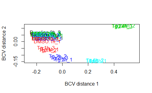
plotMDS(y, method="bcv", col=as.numeric(y$samples$group))
legend("bottomleft", as.character(unique(y$samples$group)), col=1:3, pch=20)

design <- model.matrix(~0+time, data = y$samples) 
colnames(design) <- levels(time)
rownames(design) <- colnames(y)
design
                0h 1h 24h 2h 6h
Baseline.0h_1  1  0   0  0  0
DMSO.1h_1      0  1   0  0  0
Tg.1h_1        0  1   0  0  0
DMSO.2h_1      0  0   0  1  0
Tg.2h_1        0  0   0  1  0
DMSO.6h_1      0  0   0  0  1
Tg.6h_1        0  0   0  0  1
DMSO.24h_1     0  0   1  0  0
Tg.24h_1       0  0   1  0  0
Baseline.0h_2  1  0   0  0  0
DMSO.1h_2      0  1   0  0  0
Tg.1h_2        0  1   0  0  0
DMSO.2h_2      0  0   0  1  0
Tg.2h_2        0  0   0  1  0
DMSO.6h_2      0  0   0  0  1
Tg.6h_2        0  0   0  0  1
DMSO.24h_2     0  0   1  0  0
Tg.24h_2       0  0   1  0  0
Baseline.0h_3  1  0   0  0  0
DMSO.1h_3      0  1   0  0  0
Tg.1h_3        0  1   0  0  0
DMSO.2h_3      0  0   0  1  0
Tg.2h_3        0  0   0  1  0
DMSO.6h_3      0  0   0  0  1
Tg.6h_3        0  0   0  0  1
DMSO.24h_3     0  0   1  0  0
Tg.24h_3       0  0   1  0  0
attr(,"assign")
[1] 1 1 1 1 1
attr(,"contrasts")
attr(,"contrasts")$time
[1] "contr.treatment"


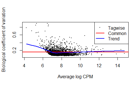
z <- estimateDisp(y,design, robust = TRUE)
sqrt(z$common.dispersion)
plotBCV(z)
plotMDS(z, labels = time)
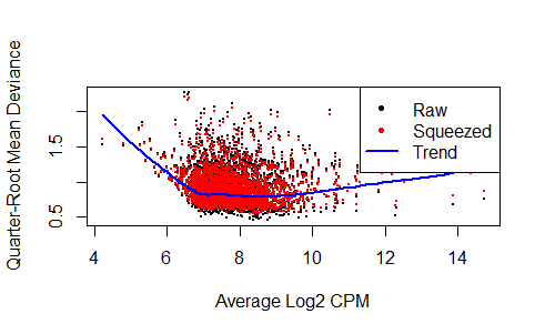
fit <- glmQLFit(z,design, robust = TRUE)
plotQLDisp(fit)

qlf <- glmQLFTest(fit,coef=1:5)
summary(decideTests(qlf))

6h-2h-24h-1h-0h
NotSig               0
Sig               3302


topTags(qlf, n=1000000)
tab2 <- as.data.frame(topTags(qlf, n=1000000)) 

Coefficient:  0h 1h 24h 2h 6h 
              genes  logFC.0h  logFC.1h logFC.24h  logFC.2h  logFC.6h   logCPM        F
Ints7            NA -12.26534 -12.27342 -12.35646 -12.28617 -12.25947 7.641854 43991.27
Cs               NA -11.58730 -11.55527 -11.53684 -11.59889 -11.56937 8.364561 42149.50
Yme1l1           NA -11.34767 -11.45401 -11.35738 -11.39468 -11.41588 8.533332 40818.42
Elavl1           NA -11.65959 -11.65544 -11.69609 -11.68613 -11.60697 8.271334 40671.67
Pdzd8            NA -11.21080 -11.16845 -11.08415 -11.22524 -11.15235 8.769288 40341.18
Rab14            NA -11.63948 -11.69195 -11.65178 -11.68748 -11.62025 8.271978 39723.03
Ppp6r3           NA -11.48140 -11.49594 -11.50953 -11.50732 -11.40042 8.453886 38766.01
Rnf14            NA -11.90126 -11.87093 -11.85145 -11.84206 -11.89443 8.063408 37941.80
Rabl6            NA -12.42685 -12.48067 -12.42238 -12.39573 -12.36443 7.515743 37101.46
Fam126b          NA -12.78592 -12.73044 -12.72118 -12.61550 -12.75967 7.217930 36670.18
Csnk2a1          NA -11.58646 -11.56253 -11.53919 -11.58012 -11.58708 8.362689 36437.87
Ube2i            NA -11.95506 -11.96058 -11.93990 -12.06529 -12.02329 7.940364 36216.62

sessionInfo( )
R version 3.6.3 (2020-02-29)
Platform: x86_64-w64-mingw32/x64 (64-bit)
Running under: Windows 10 x64 (build 19042)

Matrix products: default

locale:
[1] LC_COLLATE=English_United States.1252  LC_CTYPE=English_United States.1252   
[3] LC_MONETARY=English_United States.1252 LC_NUMERIC=C                          
[5] LC_TIME=English_United States.1252    

attached base packages:
[1] stats     graphics  grDevices utils     datasets  methods   base     

other attached packages:
[1] RColorBrewer_1.1-2 edgeR_3.28.1       limma_3.42.2      

loaded via a namespace (and not attached):
[1] compiler_3.6.3  tools_3.6.3     Rcpp_1.0.7      splines_3.6.3   grid_3.6.3     
[6] locfit_1.5-9.4  statmod_1.4.36  lattice_0.20-41

Yes, the reason why all your logFCs are negative is because you are coding the time trend incorrectly. If you had only one drug, then you would need

design <- model.matrix(~time, data = y$samples)

without the ~0 and

qlf <- glmQLFTest(fit,coef=2:5)

Removing the intercept (with ~0) is only used when you intend to form contrasts from the levels of a single factor and should not be used in any other circumstances.

However your data is more complex that this. You have an active drug (Tg) and a control (DMSO). You obviously need to include drug in the design matrix and you need to model separate time trends for the two drugs.