Question

lfcShrink MA plot comparison

0

Entering edit mode

user230613 • 0

@83d4114c

Last seen 2.5 years ago

Spain

Hello, I have just started to use DESeq2 and I am trying to compare the results obtained with and without applying lfcShrink. These are the two MA plots, one with lfcShrink and one without:

MA plot comparison

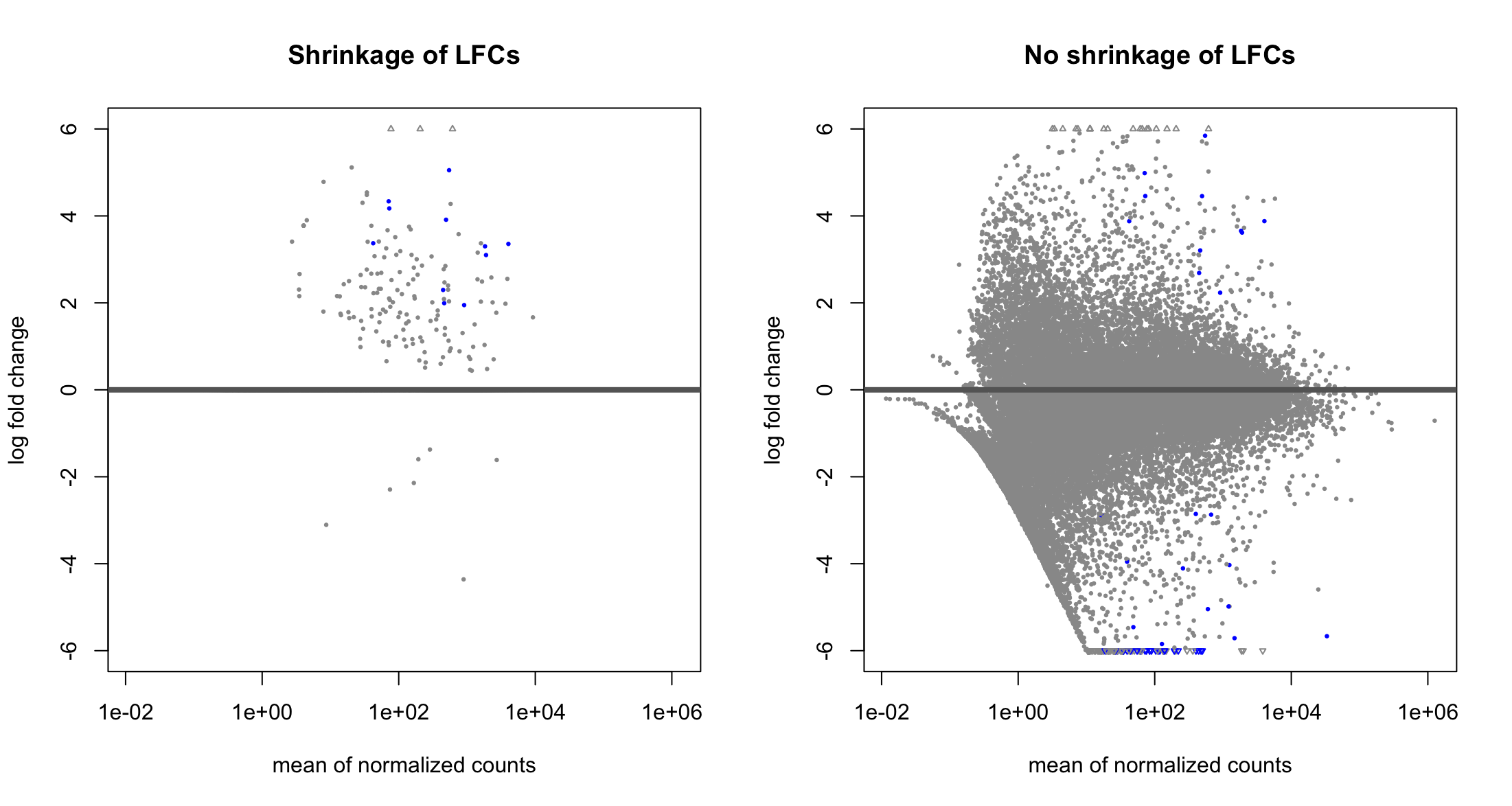
Is it normal to lose all the significant (blue) genes with negative log2FC when applying shrinkage?

I have a very unbalanced dataset, one group with approx. 25-30 samples and the other with 3. But despite this (that I know is not ideal), I would like to understand what is going on in the plots.

Summary of the results with shrinkage:

summary(resLFC)

out of 33014 with nonzero total read count
adjusted p-value < 0.1
LFC > 0 (up)       : 15, 0.045%
LFC < 0 (down)     : 33, 0.1%
outliers [1]       : 586, 1.8%
low counts [2]     : 10038, 30%
(mean count < 4)

Summary of the results without shrinkage:

summary(res)

out of 33014 with nonzero total read count
adjusted p-value < 0.1
LFC > 0 (up)       : 11, 0.033%
LFC < 0 (down)     : 37, 0.11%
outliers [1]       : 586, 1.8%
low counts [2]     : 10038, 30%
(mean count < 4)

Snippet of the commands (nothing special, just regular commands of DESeq2 afaik):

sampleTable <- data.frame(condition = samples$Responder)
dds <- DESeqDataSetFromTximport(txi, sampleTable, ~condition)
keep <- rowSums(counts(dds)) >= 10
dds <- dds[keep,]
dds = DESeq(dds)
resLFC <- lfcShrink(dds, coef=resultsNames(dds)[2], type="apeglm")

I have also posted the same question in biostars yesterday, but I figured it out that I might be more lucky posting it here :).

DESeq2 • 2.2k views

ADD COMMENT • link updated 2.6 years ago by Michael Love 42k • written 2.6 years ago by user230613 • 0

score 1 · Accepted Answer · 2022-03-22

1

Entering edit mode

Michael Love 42k

@mikelove

Last seen 5 hours ago

United States

This has been discussed previously on the support site but it's not easy to find those threads.

lfcShrink() tends to be more conservative than null hypothesis p-values that LFC = 0, especially with very small number of replicates in one group. I've seen these types of plots above for 2 vs 2 or 2 vs X. If most genes are within the range of the "noise" -- the range of the simple LFC, calculated by averaging the counts and then taking their ratio, that would be expected if LFC = 0 -- it will shrink them to 0.

If you want to avoid this you could use type="normal".

ADD COMMENT • link 2.6 years ago Michael Love 42k

0

Entering edit mode

Thanks Michael Love ! I am still a bit confused, so then it is normal that all the significant DEG with negative LFC I get without applying lfcShrink() are gone after applying lfcShrink()? Because the positive LFC hits I can see that are present in both plots, it is just the negative ones that make me concerned.

ADD REPLY • link 2.6 years ago user230613 • 0

0

Entering edit mode

Yes, well it's just that one method is more conservative at this extreme range of low sample size. Conservative meaning that p-value says the gene is of interest while the lfcShrink method is not convinced.

ADD REPLY • link 2.6 years ago Michael Love 42k

0

Entering edit mode

Another thing to notice: I'm guessing that you are comparing large vs small in your LFC right? So the denominator of the LFC is based on 2 data points? This would explain what is happening.

ADD REPLY • link 2.6 years ago Michael Love 42k

0

Entering edit mode

I see.

Actually, I am comparing the small group (responders) against the big one (non-responders). This is how the 3 MA-plots look now (without shrinkage, with apeglm and with normal). Indeed, using "normal" seems to "improve" it a bit, and I said "improve" because I don't know if it is better or not (probably not easy to assess this).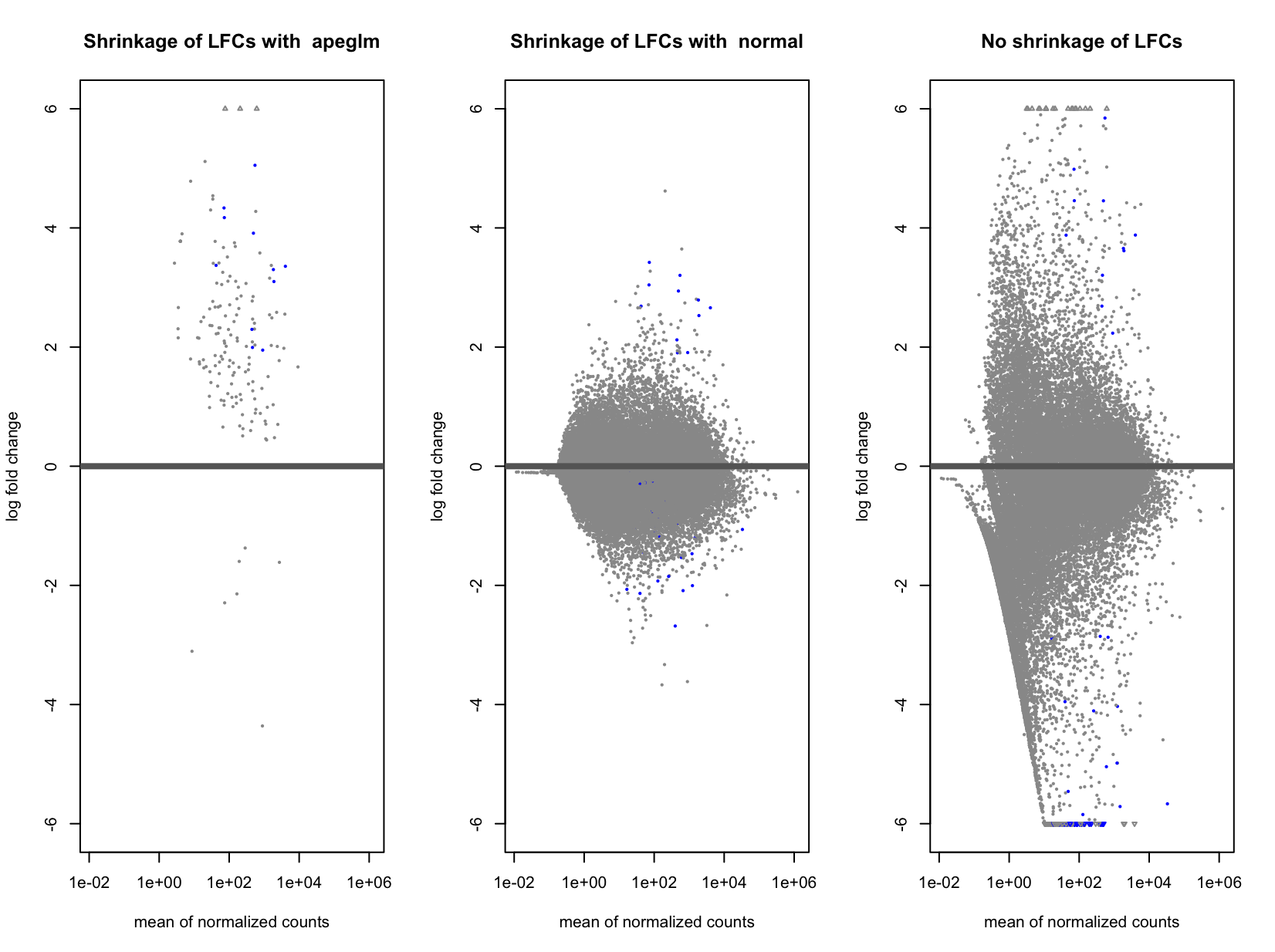 MA-plot comparison

ADD REPLY • link 2.6 years ago user230613 • 0

0

Entering edit mode

Ok if you are comparing small group (numerator) to big group (denominator) then apeglm is shrinking when you have some counts in the small group but all 0 in the big group. Does the small group have the same sequencing depth as the large group?

ADD REPLY • link 2.6 years ago Michael Love 42k

0

Entering edit mode

Exactly. Sequencing depth is the same yes. I compared a bit the results obtained using the 3 methods:

> dim(filter(as.data.frame(resLFCnorm), (!is.na(padj) & abs(log2FoldChange) >= 1 & padj <0.1)))
[1] 28  6
> dim(filter(as.data.frame(resLFCape), (!is.na(padj) & abs(log2FoldChange) >= 1 & padj <0.1)))
[1] 11  5
> dim(filter(as.data.frame(res), (!is.na(padj) & abs(log2FoldChange) >= 1 & padj <0.1)))
[1] 11
> n=filter(as.data.frame(resLFCnorm), (!is.na(padj) & abs(log2FoldChange) >= 1 & padj <0.1))
> a=filter(as.data.frame(resLFCape), (!is.na(padj) & abs(log2FoldChange) >= 1 & padj <0.1))
> r=filter(as.data.frame(res), (!is.na(padj) & abs(log2FoldChange) >= 1 & padj <0.1))
> length(intersect(rownames(n), rownames(a)))
[1] 11
> length(intersect(rownames(r), rownames(a)))
[1] 11
> length(intersect(rownames(n), rownames(r)))
[1] 28

So without shrinkage, I have highest DEGs, and using apeglm the lowest. And then, all the DEGs in apeglm, are present in normal, and present in no shrinkage.

ADD REPLY • link 2.6 years ago user230613 • 0

0

Entering edit mode

I think that normal is fine here. apeglm is conservative with very few replicates, which some would find an advantage, but you can just go with "normal".

ADD REPLY • link 2.6 years ago Michael Love 42k