Question

Confused about the CPM and TMM normalization in edgeR

2

Entering edit mode

Mohamed ▴ 30

@aa1ae679

Last seen 14 months ago

United Kingdom

I am sorry for this naive question, but is critically related to a basic step in RNA seq analyses. I am trying different normalization approach mainly CPM and TMM Assuming the following:

my raw count is named as 'counts.keep'
I am using a DGElist called 'dgeObj'

First I tried to get the log2 of just the raw count and created an object called M
M<- log2(counts.keep)

Second, I created the CPM of the log2 using the dgeObj, this object is not TMM normalized ... This creating logcounts (I assume this is the CPM of the log2 count)

logcounts <- cpm(dgeObj,log=TRUE)

Third, I tried to get the TMM normalized count, and here is my question. I used this code

dgeObj <- calcNormFactors(dgeObj)
logCPM <- cpm(dgeObj, log = TRUE)

I first make TMM normalization on the dgeObj, then used cpm function with log =TRUE on this dgeObj

What the cpm actually is doing here? is it making a cpm on top of the TMM normalized reads ? or only doing TMM ?

In another word, I would like to know if I plot the logCPM object, will this be only the TMM normalization or CPM + TMM normalization. So my confusion is can one apply CPM on top on TMM approach or normalize using only one of them to assess the normalization ?

Thanks

RNASeq R edgeR • 19k views

ADD COMMENT • link updated 3 months ago by Ahdee ▴ 50 • written 2.4 years ago by Mohamed ▴ 30

score 3 · Answer 1 · 2022-06-30

3

Entering edit mode

James W. MacDonald 67k

@james-w-macdonald-5106

Last seen 3 days ago

United States

TMM doesn't normalize the reads, but instead calculates normalization factors (hence the function name calcNormFactors). If you use cpm on a DGEList that has no normalization factors, then the logCPM values will be scale normalized using the total library size. The idea behind TMM is that there can be compositional biases, where certain genes have much higher read counts due to technical reasons, and you might not want to use them when calculating the library size. Instead of using the total library size (the sum of the reads for all genes), TMM trims off the most highly variable genes (Trimmed mean of M-values, where M-values are the log fold change between each sample and a reference) and then calculates a normalization factor that is used to adjust the library size when you compute logCPM values.

Please note that all of this information is covered in great detail in the help page for calcNormFactors, as well as in the edgeR User's Guide, and in the papers referenced in the calcNormFactors help page.

ADD COMMENT • link 2.4 years ago James W. MacDonald 67k

0

Entering edit mode

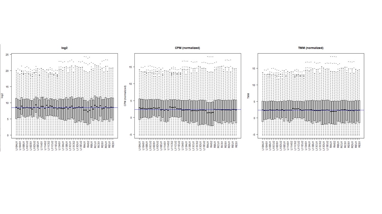
Thanks a lot. I actually understand this. My question is what happens in the resultant counts (and hence in their normalization) when using cpm on a DGEList object that have norm.factors ,,, compared to using cpm on a DGEList with no factor (factor = 1) ? I am asking this because some peoples think in the first case it is applying cpm on top of factor-corrected counts (what we might call as TMM normalization). I observed when ploting log2, cpm, cpm + TMM, that normalization is gettting better . see image Comparison between normalization effect

Also ca you advice on any other way to test if certain normalization is performing better that other ?

Thanks

ADD REPLY • link 2.4 years ago Mohamed ▴ 30

0

Entering edit mode

I just explained how it works, and you told me you understand all that, but then ask the same question all over again? Perhaps you should re-read my post and the help page I pointed you towards.

Also there is no way to 'test if a certain normalization is performing better' because we don't know the underlying truth. We make assumptions that seem reasonable and then go forward with the analysis. And when you present your results you say what you did, and perhaps why you think it was a reasonable thing to do.

ADD REPLY • link 2.4 years ago James W. MacDonald 67k

0

Entering edit mode

Sorry for misunderstanding. What I meant was that there is always two option of using cpm on DGElist as shown in my above codes: Option 1: make cpm on DGE list with the normalization factor being 1 (so before making: dgeObj <- calcNormFactors(dgeObj) Option 2: make cpm on DGElist after performing TMM, when we have normalization factors shown in the sample slot of the DGElist (so after applying this : dgeObj <- calcNormFactors(dgeObj))

So my question was what is the difference in terms of the resultant counts between both options ? and when visualizing that ?. in the boxplot shown above, the 2nd one is when option 1 applies, and the 3rd one is when option 2 applies. I could observe that with cpm on a TMM normalized subjects it is better normalized (so the middle blue median line is almost similar to the black median line of all libraries)... For me the differences between 2 and 3 rd box plot indicate difference underlying counts >> am I right ?

ADD REPLY • link 2.4 years ago Mohamed ▴ 30

0

Entering edit mode

calcNormFactors normalizes the library sizes.

cpm divides counts by library sizes.

Running cpm after calcNormFactors uses normalized library sizes. Running cpm before calcNormFactors uses unnormalized library sizes. Obviously the former is better than the latter. Why would you normalize the library sizes but then ignore the normalization? That would just make no sense at all.

ADD REPLY • link 14 months ago Gordon Smyth 52k

score 0 · Answer 2 · 2022-06-30

0

Entering edit mode

Gordon Smyth 52k

@gordon-smyth

Last seen 8 minutes ago

WEHI, Melbourne, Australia

There's no such thing as TMM normalized counts, as the edgeR document tells you. This link might help: https://www.biostars.org/p/9475236/