My dataset has a total of 53 samples (with outliers removed) of breast cancer patients with two conditions.
I have read that DESeq2 doesn’t provide automatic shrinkage, and I have to use lfcShrink to shrink the log2FoldChanges. The manual states that apeGLM and ashr perform better than the normal option and that apeGLM is quite strict compared to the others and performs well with small samples.
Default options on everything : Over 60% of genes are flagged as outliers.
  dds <- DESeqDataSetFromMatrix(countData = round(filtered_counts),
                                    colData = filtered_coldata,
                                    design = ~ condition)

  dds <- DESeq(dds)
    ## estimating size factors
    ## estimating dispersions
    ## gene-wise dispersion estimates
    ## mean-dispersion relationship
    ## final dispersion estimates
    ## fitting model and testing
    ## -- replacing outliers and refitting for 18774 genes
    ## -- DESeq argument 'minReplicatesForReplace' = 7
    ## -- original counts are preserved in counts(dds)
    ## estimating dispersions
    ## fitting model and testing
res <- results(dds)
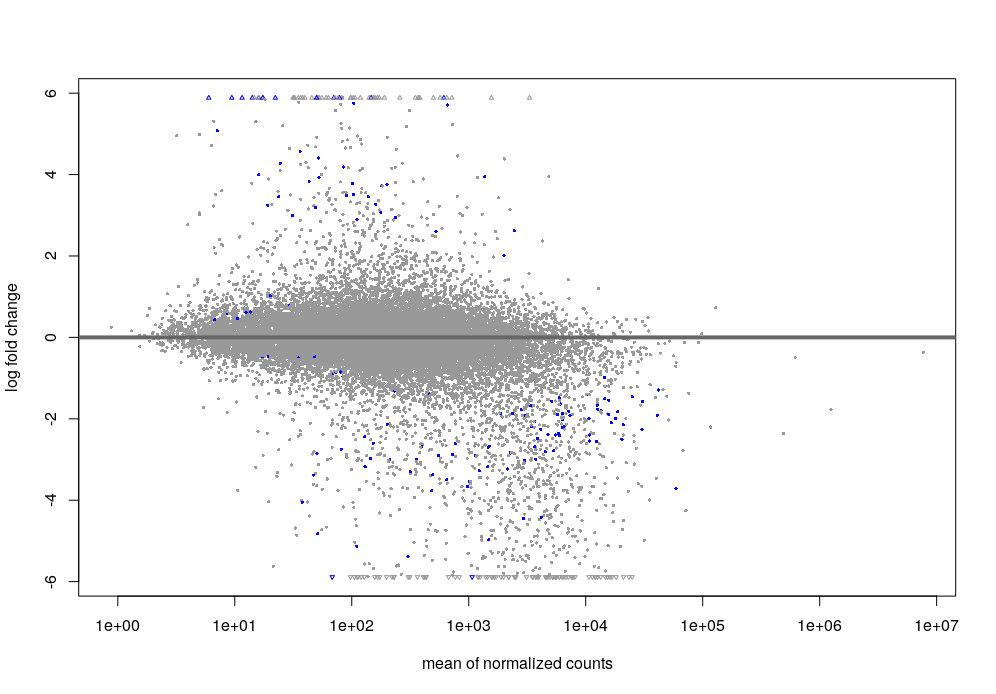
The MA plot with the results looks like this.
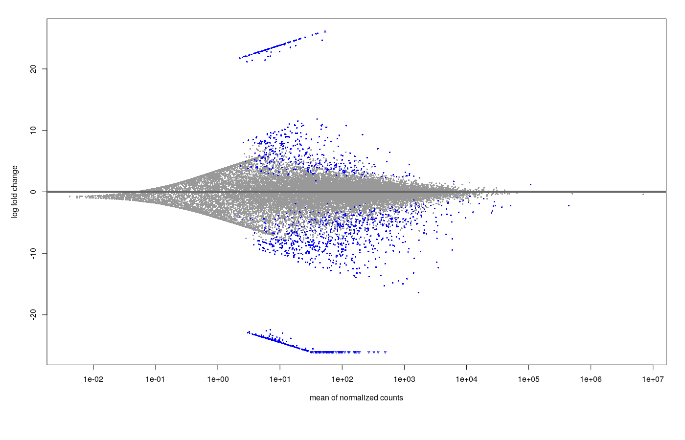
- Shrinkage (ashr) MA plot
- Shrinkage (apeGLM) MA plot
I saw this post and response so I also tried subsetting off a number of the small count genes.
    keep <- rowSums(counts(dds) >= 10) >= 5
    table(keep)
    dds <- dds[keep,]
- Default DESeq: after shrinkage (apeGLM), the MA plot looks like this.
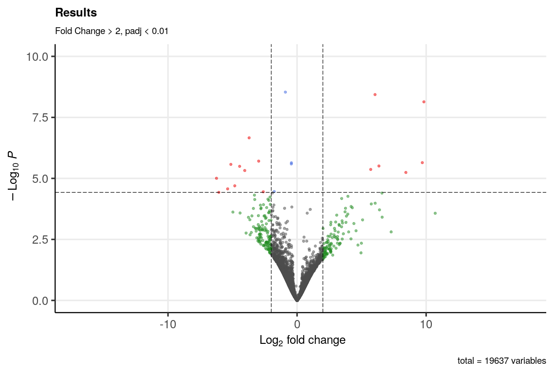
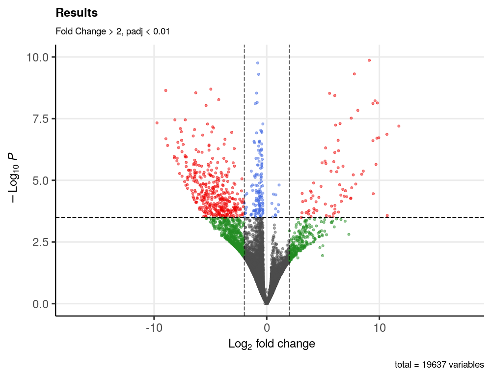
And the volcano plot looks like this.
- minRep = Inf and cooksCutoff = F : after shrinkage (apeGLM), the MA plot looks like this.
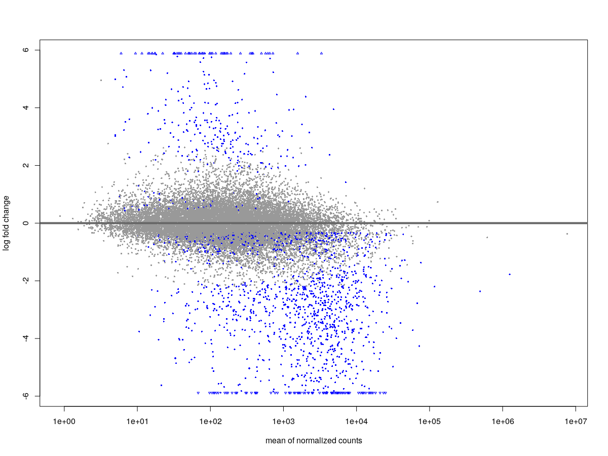
Ultimately, my questions are:
Why are so many genes flagged as outliers? I have performed additional inspection of the data but nothing really suggests particular samples as outliers. Would this suggest there is something wrong with the data?
Should I be using minRep = Inf and cooksCutoff = F? I saw that with large datasets, this is sometimes preferred. If then, why are these turned on as the default? Is it useful for smaller datasets?
Is performing shrinkage the best way to proceed? I don’t really understand fully what shrinkage does, as it seems to not only affect the visualisation but also which genes are found significant.
For the shrinkage, is apeGLM the best way to go even with larger datasets, or is it only appropriate for small datasets?
Sorry for all the questions but I have no background in bioinformatics and really struggling to understand log2FoldChange shrinkage methods.
sessionInfo()


R version 4.2.0 (2022-04-22)
Platform: x86_64-pc-linux-gnu (64-bit)
Running under: Ubuntu 20.04.4 LTS

Matrix products: default
BLAS:   /usr/lib/x86_64-linux-gnu/openblas-pthread/libblas.so.3
LAPACK: /usr/lib/x86_64-linux-gnu/openblas-pthread/liblapack.so.3

locale:
 [1] LC_CTYPE=en_US.UTF-8       LC_NUMERIC=C               LC_TIME=en_US.UTF-8        LC_COLLATE=en_US.UTF-8
 [5] LC_MONETARY=en_US.UTF-8    LC_MESSAGES=en_US.UTF-8    LC_PAPER=en_US.UTF-8       LC_NAME=C
 [9] LC_ADDRESS=C               LC_TELEPHONE=C             LC_MEASUREMENT=en_US.UTF-8 LC_IDENTIFICATION=C

attached base packages:
[1] stats4    stats     graphics  grDevices utils     datasets  methods   base

other attached packages:
 [1] ashr_2.2-54                 ggfortify_0.4.14            Rcpp_1.0.9                  tibble_3.1.8
 [5] dplyr_1.0.9                 EnhancedVolcano_1.14.0      ggrepel_0.9.1               clusterProfiler_4.4.4
 [9] msigdbr_7.5.1               fgsea_1.22.0                tximport_1.24.0             data.table_1.14.2
[13] biomaRt_2.52.0              ggplot2_3.3.6               DESeq2_1.36.0               SummarizedExperiment_1.26.1
[17] Biobase_2.56.0              MatrixGenerics_1.8.1        matrixStats_0.62.0          GenomicRanges_1.48.0
[21] GenomeInfoDb_1.32.2         IRanges_2.30.0              S4Vectors_0.34.0            BiocGenerics_0.42.0

loaded via a namespace (and not attached):
  [1] shadowtext_0.1.2       fastmatch_1.1-3        BiocFileCache_2.4.0    plyr_1.8.7             igraph_1.3.4
  [6] lazyeval_0.2.2         splines_4.2.0          BiocParallel_1.30.3    digest_0.6.29          invgamma_1.1
 [11] yulab.utils_0.0.5      htmltools_0.5.3        GOSemSim_2.22.0        viridis_0.6.2          GO.db_3.15.0
 [16] SQUAREM_2021.1         fansi_1.0.3            magrittr_2.0.3         memoise_2.0.1          Biostrings_2.64.0
 [21] annotate_1.74.0        graphlayouts_0.8.0     bdsmatrix_1.3-6        enrichplot_1.16.1      prettyunits_1.1.1
 [26] colorspace_2.0-3       apeglm_1.18.0          blob_1.2.3             rappdirs_0.3.3         xfun_0.31
 [31] crayon_1.5.1           RCurl_1.98-1.8         jsonlite_1.8.0         scatterpie_0.1.7       genefilter_1.78.0
 [36] survival_3.3-1         ape_5.6-2              glue_1.6.2             polyclip_1.10-0        gtable_0.3.0
 [41] zlibbioc_1.42.0        XVector_0.36.0         DelayedArray_0.22.0    scales_1.2.0           DOSE_3.22.0
 [46] mvtnorm_1.1-3          DBI_1.1.3              emdbook_1.3.12         viridisLite_0.4.0      xtable_1.8-4
 [51] progress_1.2.2         gridGraphics_0.5-1     tidytree_0.3.9         bit_4.0.4              DT_0.23
 [56] truncnorm_1.0-8        htmlwidgets_1.5.4      httr_1.4.3             RColorBrewer_1.1-3     ellipsis_0.3.2
 [61] pkgconfig_2.0.3        XML_3.99-0.10          farver_2.1.1           dbplyr_2.2.1           locfit_1.5-9.6
 [66] utf8_1.2.2             labeling_0.4.2         ggplotify_0.1.0        tidyselect_1.1.2       rlang_1.0.4
 [71] reshape2_1.4.4         AnnotationDbi_1.58.0   munsell_0.5.0          tools_4.2.0            cachem_1.0.6
 [76] downloader_0.4         cli_3.3.0              generics_0.1.3         RSQLite_2.2.15         evaluate_0.15
 [81] stringr_1.4.0          fastmap_1.1.0          yaml_2.3.5             ggtree_3.4.1           babelgene_22.3
 [86] knitr_1.39             bit64_4.0.5            tidygraph_1.2.1        purrr_0.3.4            KEGGREST_1.36.3
 [91] ggraph_2.0.5           nlme_3.1-157           aplot_0.1.6            DO.db_2.9              xml2_1.3.3
 [96] compiler_4.2.0         rstudioapi_0.13        plotly_4.10.0          filelock_1.0.2         curl_4.3.2
[101] png_0.1-7              treeio_1.20.1          tweenr_1.0.2           geneplotter_1.74.0     stringi_1.7.8
[106] lattice_0.20-45        Matrix_1.4-1           vctrs_0.4.1            pillar_1.8.0           lifecycle_1.0.1
[111] irlba_2.3.5            bitops_1.0-7           patchwork_1.1.1        qvalue_2.28.0          R6_2.5.1
[116] gridExtra_2.3          codetools_0.2-18       MASS_7.3-57            assertthat_0.2.1       withr_2.5.0
[121] GenomeInfoDbData_1.2.8 parallel_4.2.0         hms_1.1.1              grid_4.2.0             ggfun_0.0.6
[126] coda_0.19-4            tidyr_1.2.0            rmarkdown_2.14         bbmle_1.0.25           mixsqp_0.3-43
[131] ggforce_0.3.3          numDeriv_2016.8-1.1

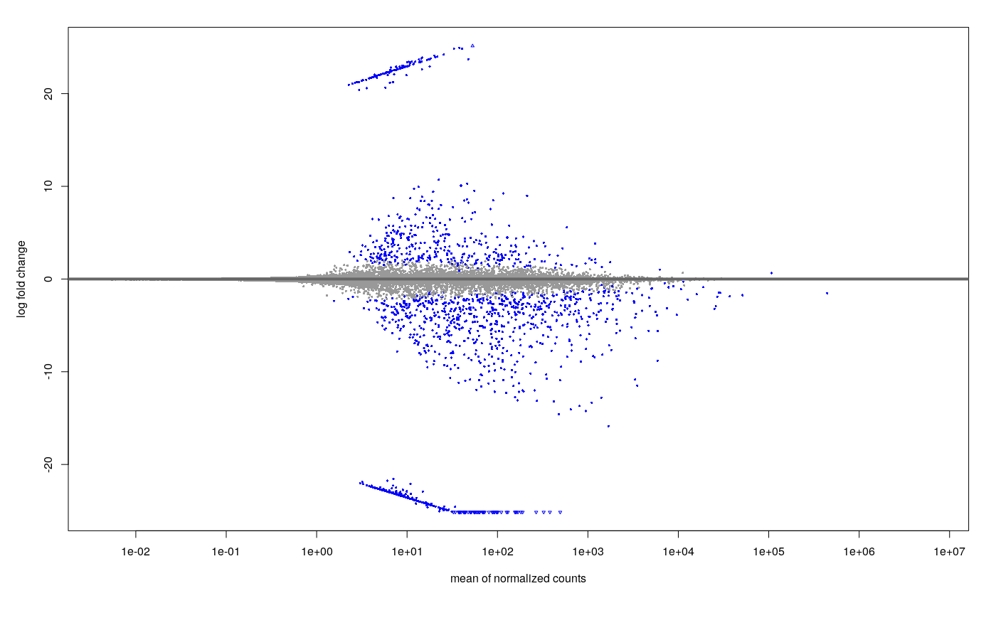
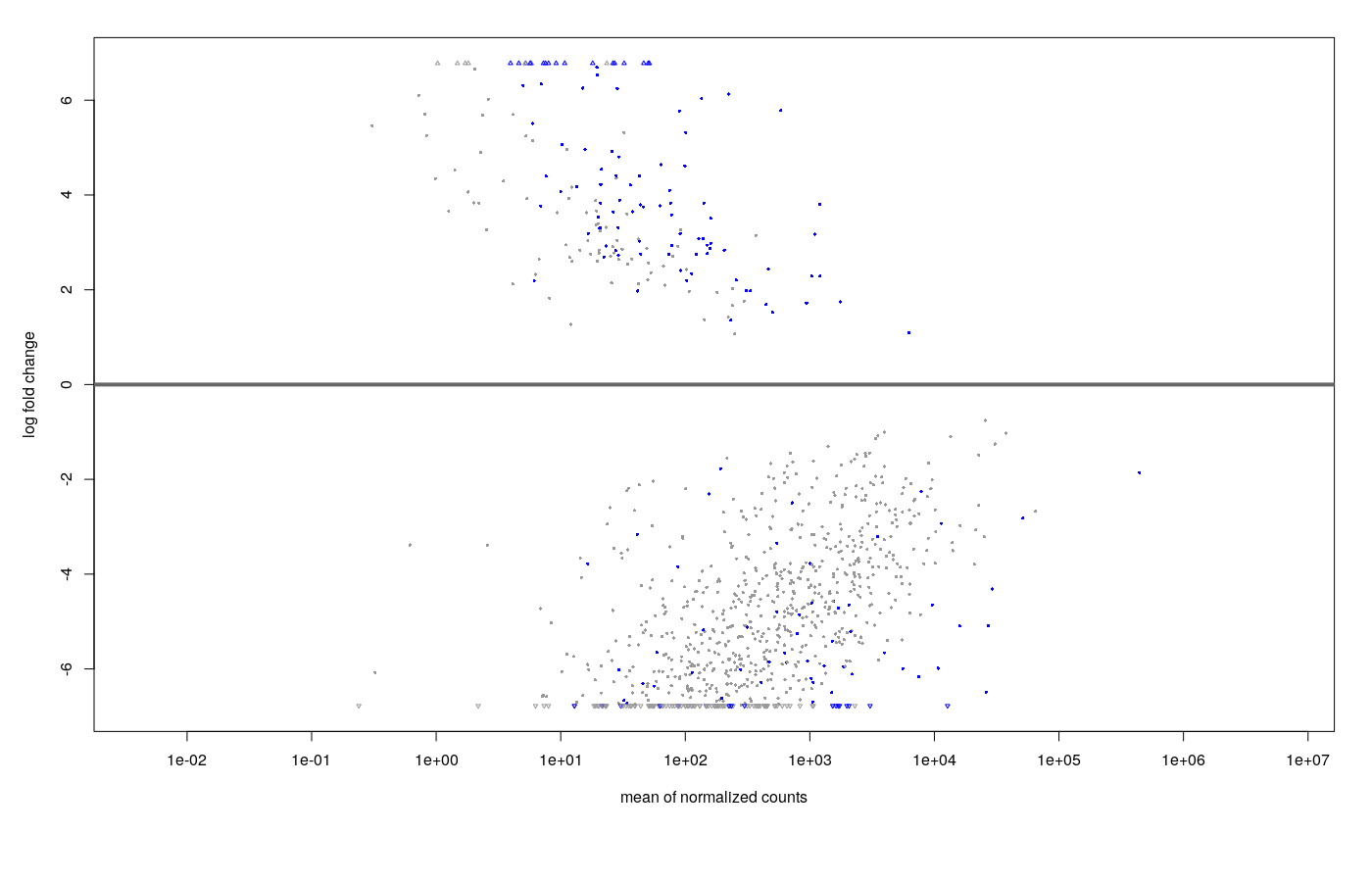

I did use plotCounts and nothing really stood out which is confusing me. I will try to inspect more samples and genes though! It does seem that the low count gene filter is definitely the way to go here! I guess if the shrinkage doesn't affect the padj then it must only be the log2FoldChange that affected my results, I was just taken aback by how different the results were. Thanks so much for your answer :)
If possible, could you explain how apeGLM and ashr are different? I know that their statistical methods are different, but I'm not sure which one to use in which situation (sample size, dispersion, etc.). Perhaps my statistical knowledge is not enough to understand how these methods affect the data.
There is an "extended section on shrinkage" in the vignette to check out. Briefly, ashr has a flexible prior but relies on the normal distribution for the coefficient, while apeglm has a fixed shape of prior (Cauchy) and uses the likelihood directly. It's a bit subtle the difference. It's hard for me to predict though when one will have a particular behavior compared to the other. You can just visualize both and assess which seems to give better shrinkage while retaining the rank of the reliable differences.
okay intresting