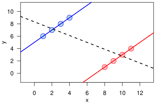
Dear all, I performed a differential gene expression analysis with the DESeq2 package and corrected for hidden variation with the sva package. Now I found genes, which have a negative LFC value in response to a given treatment, although they have higher (normalized) counts in these treatment samples than in the control samples. These genes are not significantly expressed in this treatment, but they show a significant interaction between two factors and I was wondering whether I can trust the interaction term, when the sign of the ES might be wrong/biased? When I check the expression of this gene in the data set which is not corrected with sva, then the LFC in the single factor treatment is positive (still not significant), as I would expect based on the counts. I thought that the covariates will correct for data variation that is not related to the treatment but I did not expect that this might result in a change of the effect size sign?
Any thoughts on that are very much appreciated :)!
Here are the relevant code snippets
##create DESeq object
dds1 <- DESeqDataSetFromTximport(txi.sum, sampleData, design= ~ Salt*Sediment*Flow)
dds1 <- DESeq(dds1)

##estimate SVs
dat  <- counts(dds1, normalized = TRUE)
mod  <- model.matrix(~ Salt*Sediment*Flow, colData(dds1)) ##full model
mod0 <- model.matrix(~   1, colData(dds1))
svseq <- svaseq(dat, mod, mod0)   #this estimated 10 SVs

#include SVs

ddssva <- dds1
ddssva$SV1 <- svseq$sv[,1]
ddssva$SV2 <- svseq$sv[,2]
ddssva$SV3 <- svseq$sv[,3]
ddssva$SV4 <- svseq$sv[,4]
ddssva$SV5 <- svseq$sv[,5]
ddssva$SV6 <- svseq$sv[,6]
ddssva$SV7 <- svseq$sv[,7]
ddssva$SV8 <- svseq$sv[,8]
ddssva$SV9 <- svseq$sv[,9]
ddssva$SV10 <- svseq$sv[,10]

design(ddssva) <- ~ SV1+SV2+SV3+SV4+SV5+SV6+SV7+SV8+SV9+SV10+Salt*Sediment*Flow
ddssva <- DESeq(ddssva)

##genes which show a different expression due to the interaction of sediment and flow
sed_flow_inter <- results(ddssva, contrast = list(c("Sedimentadded.Flowreduced")), alpha = sig_lvl)

##extract results for the single treatment
flow <- results(ddssva, contrast=c("Flow.Velocity", "reduced", "normal"), alpha = sig_lvl)


sessionInfo( )

R version 4.1.1 (2021-08-10)
Platform: x86_64-w64-mingw32/x64 (64-bit)
Running under: Windows 10 x64 (build 19044)

Matrix products: default

locale:
[1] LC_COLLATE=German_Germany.1252  LC_CTYPE=German_Germany.1252
[3] LC_MONETARY=German_Germany.1252 LC_NUMERIC=C
[5] LC_TIME=German_Germany.1252

attached base packages:
[1] parallel  stats4    stats     graphics  grDevices utils
[7] datasets  methods   base

other attached packages:
 [1] DEGreport_1.28.0            ashr_2.2-54
 [3] apeglm_1.14.0               PCAtools_2.4.0
 [5] ggrepel_0.9.1               ggplot2_3.3.6
 [7] sva_3.40.0                  BiocParallel_1.26.2
 [9] genefilter_1.74.1           mgcv_1.8-36
[11] nlme_3.1-152                DESeq2_1.32.0
[13] SummarizedExperiment_1.22.0 Biobase_2.52.0
[15] MatrixGenerics_1.4.3        matrixStats_0.62.0
[17] GenomicRanges_1.44.0        GenomeInfoDb_1.28.4
[19] IRanges_2.26.0              S4Vectors_0.30.2
[21] BiocGenerics_0.38.0         tximport_1.20.0

loaded via a namespace (and not attached):
  [1] colorspace_2.0-3            rjson_0.2.21
  [3] ellipsis_0.3.2              circlize_0.4.15
  [5] XVector_0.32.0              ggdendro_0.1.23
  [7] GlobalOptions_0.1.2         clue_0.3-61
  [9] rstudioapi_0.13             bit64_4.0.5
 [11] AnnotationDbi_1.54.1        fansi_1.0.3
 [13] mvtnorm_1.1-3               codetools_0.2-18
 [15] splines_4.1.1               sparseMatrixStats_1.4.2
 [17] logging_0.10-108            mnormt_2.1.0
 [19] doParallel_1.0.17           cachem_1.0.6
 [21] knitr_1.39                  geneplotter_1.70.0
 [23] Nozzle.R1_1.1-1.1           broom_1.0.0
 [25] annotate_1.70.0             cluster_2.1.2
 [27] png_0.1-7                   compiler_4.1.1
 [29] httr_1.4.3                  backports_1.4.1
 [31] dqrng_0.3.0                 assertthat_0.2.1
 [33] Matrix_1.3-4                fastmap_1.1.0
 [35] limma_3.48.3                cli_3.3.0
 [37] BiocSingular_1.8.1          lasso2_1.2-22
 [39] tools_4.1.1                 rsvd_1.0.5
 [41] coda_0.19-4                 gtable_0.3.0
 [43] glue_1.6.2                  GenomeInfoDbData_1.2.6
 [45] reshape2_1.4.4              dplyr_1.0.9
 [47] Rcpp_1.0.9                  bbmle_1.0.25
 [49] vctrs_0.4.1                 Biostrings_2.60.2
 [51] iterators_1.0.14            DelayedMatrixStats_1.14.3
 [53] psych_2.2.5                 xfun_0.31
 [55] stringr_1.4.0               beachmat_2.8.1
 [57] lifecycle_1.0.1             irlba_2.3.5
 [59] XML_3.99-0.10               edgeR_3.34.1
 [61] zlibbioc_1.38.0             MASS_7.3-54
 [63] scales_1.2.0                RColorBrewer_1.1-3
 [65] ComplexHeatmap_2.11.1       memoise_2.0.1
 [67] emdbook_1.3.12              bdsmatrix_1.3-6
 [69] reshape_0.8.9               stringi_1.7.6
 [71] RSQLite_2.2.14              SQUAREM_2021.1
 [73] foreach_1.5.2               ScaledMatrix_1.0.0
 [75] shape_1.4.6                 truncnorm_1.0-8
 [77] rlang_1.0.4                 pkgconfig_2.0.3
 [79] bitops_1.0-7                lattice_0.20-44
 [81] invgamma_1.1                purrr_0.3.4
 [83] cowplot_1.1.1               bit_4.0.4
 [85] tidyselect_1.1.2            plyr_1.8.7
 [87] magrittr_2.0.3              R6_2.5.1
 [89] generics_0.1.3              DelayedArray_0.18.0
 [91] DBI_1.1.3                   pillar_1.7.0
 [93] withr_2.5.0                 survival_3.2-11
 [95] KEGGREST_1.32.0             RCurl_1.98-1.7
 [97] mixsqp_0.3-43               tibble_3.1.7
 [99] crayon_1.5.1                utf8_1.2.2
[101] GetoptLong_1.0.5            locfit_1.5-9.6
[103] grid_4.1.1                  blob_1.2.3
[105] ConsensusClusterPlus_1.56.0 digest_0.6.29
[107] xtable_1.8-4                tidyr_1.2.0
[109] numDeriv_2016.8-1.1         munsell_0.5.0


Thanks a lot!