All genes in a set for gseGO funtion
1
1
Entering edit mode
Adelyn ▴ 10
@47ceacfa
Last seen 2.2 years ago
United States

Hello,

I am using gseGO to determine the pathways impacted by the differential expression I am seeing. It returns the pathway (GO Term), the percentage of genes impacted and the setSize. I want to find the other genes in the set. So say it give 60% of genes in a GO term with a set size of 100 are impacted, I want to know what the other 40 genes are.

Is there a way to access the what is in the set for each GO term specific to gseGO?

I can find all genes/gene products associated with GO terms, but these lists do not match the set size given by gseGO.

Thank you for your help, Adelyn

gseGO setSize • 5.0k views
ADD COMMENT
0
Entering edit mode

You indicated that you are able to find all genes associated with a GO term, but did you then filter out the genes that are not in your dataset?

Also, showing the code you used would be helpful.

ADD REPLY
0
Entering edit mode

I use:

    library(clusterProfiler)
library(enrichplot)
library(ggplot2)
install.packages("ggnewscale")
require(DOSE)
install.packages("ggridges")
organism="org.Mm.eg.db"
#ENSEMBL ID
df = read.csv("ALL.csv", header=TRUE)
original_gene_list <- df$logFC
names(original_gene_list) <- df$Geneid
gene_list<-na.omit(original_gene_list)
gene_list = sort(gene_list, decreasing = TRUE)
#FDR all
gse <- gseGO(geneList=gene_list, ont ="ALL", keyType = "ENSEMBL", minGSSize = 3, maxGSSize = 1000, pvalueCutoff = 0.05, verbose = TRUE, OrgDb = organism, pAdjustMethod = "fdr", nPermSimple = 100000)
df <-data.frame(gse)
write.csv(df,"GSE_All.csv", row.names = TRUE)

I then get an csv that gives: enter image description here Where I get the genes impacted in the set under core_enrichment, but this is only 15% of the genes in a set of 430. I want to find the other 365 terms that were not impacted. This would make a complete the list associated with the GO term specific to this gseGO function's GO term. But I have yet to find a way to give me that.

If I use:

z <- mapIds(org.Mm.eg.db, keys(org.Mm.eg.db, "GO"), "ENSEMBL", "GO", multiVals = "list")
lapply(z[1:4], head)

zz <- select(org.Mm.eg.db, keys(org.Mm.eg.db, "GO"), "ENSEMBL", "GO")
#'select()' returned 1:many mapping between keys and columns
head(zz)
df <-data.frame(zz)

To get a complete list of mapped GO terms and ensembl IDs, the # of genes do not match the setSize when looking at a particular GO term and sometime not all the core_enrichment genes are listed.

ADD REPLY
0
Entering edit mode
@james-w-macdonald-5106
Last seen 3 days ago
United States

clusterProfiler does exactly what you have done, and then passes those data on to the fgsea package, which then apparently filters out some of the genes. It's not clear to me when/why that happens, but maybe the maintainer of fgsea will provide an answer.

I should also point out that using Ensembl Gene IDs in this context is problematic. What will happen is the Ensembl Gene IDs will first be mapped to NCBI Gene IDs, and then those will be used to map to GO terms. This is unavoidable if you use an OrgDb, because the underlying database has NCBI Gene IDs as the central key, so any query between tables is mapped via the NCBI Gene ID. Anyway, the first step is quite frail, as EBI/EMBL and NCBI do not agree on which genes are the same, so you will silently drop genes at that first step.

As a super simple example, here's how many Ensembl Gene IDs cannot be mapped

> library(org.Mm.eg.db)
> mapper <- mapIds(org.Mm.eg.db, keys(org.Mm.eg.db), "ENSEMBL", "ENTREZID", multiVals = "list")
'select()' returned 1:many mapping between keys and columns
> nagns <- names(mapper)[sapply(mapper, function(x) all(is.na(x)))]
> length(nagns)
[1] 40079
> length(nagns)/length(mapper)
[1] 0.5484189
## Ooof

## how many of those NCBI Gene IDs does EBI/EMBL map?
> library(biomaRt)
> mart <- useEnsembl("ensembl","mmusculus_gene_ensembl")
> ensmap <- getBM(c("ensembl_gene_id","entrezgene_id"), "entrezgene_id", nagns, mart)
> head(ensmap)
     ensembl_gene_id entrezgene_id
1 ENSMUSG00000102439         14246
2 ENSMUSG00000121135         15365
3 ENSMUSG00000070645         19702
4 ENSMUSG00000107355        100740
5 ENSMUSG00000120083         67644
6 ENSMUSG00000085385         68108
> dim(ensmap)
[1] 217   2

So NCBI only maps ~45% of their IDs to Ensembl IDs, and of those that don't map, Ensembl says 217 DO map. You can do the converse (use biomaRt to map Ensembl IDs to NCBI Gene IDs) and you will get a different set of genes that do/don't map.

Anyway, long story short, you would be better served if you could work with NCBI Gene IDs throughout.

ADD COMMENT
0
Entering edit mode

Thank you for the help with the gene ID issue. The raw counts file is in Ensembl IDs which I map to Entrez IDs to do the DGE analysis. I switch back in this case because I know they all map, and its easier to use online tool to spit out the gene symbols which are easier to understand for my human brain. But I will keep consistency in mind.

Any ideas on why the GO database list of gene for a certain GO term do not match the tags gseGO implicates for a certain pathway?

ADD REPLY
0
Entering edit mode

You would have to provide an example.

ADD REPLY
0
Entering edit mode

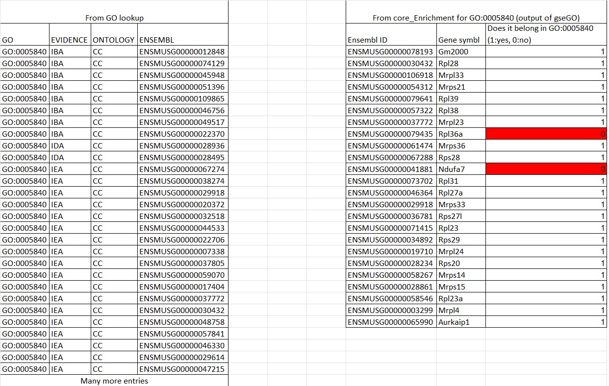
Take GO:0005840 for example:

gseGO results give a setSize of 28, Leading edge stats of tags=86%, list=22%, signal=69%, and the list of genes on the right (where there are 24 genes with agrees with 86% of tags enriched).

Looking up the GO term via the z<-mapIds(....) code above I get a long list of 178 unique genes on the left.

Comparing to see if the genes spit out by gseGO are in the GO:0005840 database from z<-mapIds code, there are 2 genes that don't appear in the database lookup. Why is this?

Also the setSize, which I assumed to be the number of genes associated with GO:0005840 is way lower than the 178 genes associated with database entry.

My goal initially was to look into the negative space (genes not leading to enrichment). So in this example,

  1. I would like to find the other 4 genes belonging to the setSize of 28
  2. In addition, I would like to understand where gseGO is getting that these 2 terms highlighted in red lead to enrichment
  3. and why the setSize differs from the number of gene associated with the GO term in the database

Thank you for your help, Adelyn

enter image description here

ADD REPLY
0
Entering edit mode

This is the part I was talking about earlier. I actually get 231 genes for that GO term. And if we run gseGO under the debugger, that's what we get as well.

> debug(gseGO)
## fake up a geneList object just so we can get gseGO to run
> rando <- runif(20) * 10
> rando <- sort(rando, decreasing = TRUE)
## fake geneList
> geneList <- setNames(rando, head(keys(org.Mm.eg.db, "ENSEMBL"), 20))
## run under debugger
> gseGO(geneList, "CC", org.Mm.eg.db, "ENSEMBL")
debugging in: gseGO(geneList, "CC", org.Mm.eg.db, "ENSEMBL")
debug: {
    ont %<>% toupper
    ont <- match.arg(ont, c("BP", "MF", "CC", "ALL"))
    GO_DATA <- get_GO_data(OrgDb, ont, keyType)
    res <- GSEA_internal(geneList = geneList, exponent = exponent, 
        minGSSize = minGSSize, maxGSSize = maxGSSize, eps = eps, 
        pvalueCutoff = pvalueCutoff, pAdjustMethod = pAdjustMethod, 
        verbose = verbose, USER_DATA = GO_DATA, seed = seed, 
        by = by, ...)
    if (is.null(res)) 
        return(res)
    if (keyType == "SYMBOL") {
        res@readable <- TRUE
    }
    res@organism <- get_organism(OrgDb)
    res@setType <- ont
    res@keytype <- keyType
    if (ont == "ALL") {
        res <- add_GO_Ontology(res, GO_DATA)
    }
    return(res)
}
Browse[2]> 
debug: ont %<>% toupper
Browse[2]> 
debug: ont <- match.arg(ont, c("BP", "MF", "CC", "ALL"))
Browse[2]> 
debug: GO_DATA <- get_GO_data(OrgDb, ont, keyType)            <------------------- We step through until this object is created
Browse[2]> 
debug: res <- GSEA_internal(geneList = geneList, exponent = exponent, 
    minGSSize = minGSSize, maxGSSize = maxGSSize, eps = eps, 
    pvalueCutoff = pvalueCutoff, pAdjustMethod = pAdjustMethod, 
    verbose = verbose, USER_DATA = GO_DATA, seed = seed, by = by, 
    ...)

## GO_DATA is an environment. Let's see what's in there
Browse[2]> ls(GO_DATA)
[1] "EXTID2PATHID" "GO2ONT"       "PATHID2EXTID" "PATHID2NAME" 

## I've poked around enough to know we want the third item
Browse[2]> z <- get("PATHID2EXTID", GO_DATA)
Browse[2]> length(z$`GO:0005840`)
[1] 231

The next step is to send this object on to GSEA_internal, which by default will pass it on to fgsea. At which point the number of genes for that GO term apparently get cut down somehow. I don't really know how/why, and am not really that interested, as GSEA IMO has been long surpassed by more powerful/useful methods. If I wanted to do a GO analysis I would use GOstats or goseq (for RNA-Seq data), and otherwise would tend to do a self-contained gene set test using roast or fry, because I understand how they work, and it makes sense to me.

ADD REPLY
1
Entering edit mode

@James: Interesting discussion and findings... but is this cutting down not simply due to the fact that some genes that belong to a GO term are not present in the data set? This is also what I meant with my initial comment above, and seems to be corroborated by this thread at the fgsea developer's site ("fgsea filters out all of the genes [from the gene sets], not present in the ranking. You don't have to do it manually.") https://github.com/ctlab/fgsea/issues/119

Maybe the TS could check this out for a GO term?

ADD REPLY
1
Entering edit mode

Hey Guido, that's probably got something to do with it. And the mapping between Ensembl and NCBI Gene IDs.

ADD REPLY
1
Entering edit mode

I had a look at it, and I concluded the cutting down of the sizes of the GO terms is indeed due to the fact that some GO term genes are not present in the dataset. I could fully reproduce the numbers in the output of gseGO. For this I used some included example data. Note that this is example data is entrez id-based, but the same would apply to an ensembl id-based gene list.

Two other remarks: when looking up genes annotated to a GO term (via the z<-mapIds(....) code above; first post), you should query for GOALL, not GO. GO includes only GO terms that are directly appended to a gene, and GOALL includes the direct term as well as their ancestors. See e.g. what's the difference between this two AnnotationDbi::select type in GO select

Also: it is recommended to replace the permutation mode of gseGO by the exact p-value calculations implemented in fgsea.

> set.seed(1234) ## for reproducibility
> 
> library(clusterProfiler)
> library(org.Hs.eg.db)
>  
> data(geneList, package="DOSE") ## use example data (for reproducibility)
> 
> # run gseGO
> gse <- gseGO(
+   geneList = geneList,
+   ont = "ALL",
+   OrgDb = org.Hs.eg.db,
+   keyType = "ENTREZID",
+   minGSSize = 3,
+   maxGSSize = 1000,
+   eps = 0,
+   pvalueCutoff = 0.05,
+   pAdjustMethod = "fdr",
+   seed = TRUE)
preparing geneSet collections...
GSEA analysis...
leading edge analysis...
done...
> 
> # check
> gse
#
# Gene Set Enrichment Analysis
#
#...@organism    Homo sapiens 
#...@setType     GOALL 
#...@keytype     ENTREZID 
#...@geneList    Named num [1:12495] 4.57 4.51 4.42 4.14 3.88 ...
 - attr(*, "names")= chr [1:12495] "4312" "8318" "10874" "55143" ...
#...nPerm        
#...pvalues adjusted by 'fdr' with cutoff <0.05 
#...844 enriched terms found
'data.frame':   844 obs. of  12 variables:
 $ ONTOLOGY       : chr  "BP" "BP" "BP" "BP" ...
 $ ID             : chr  "GO:0000278" "GO:1903047" "GO:0000819" "GO:0007059" ...
 $ Description    : chr  "mitotic cell cycle" "mitotic cell cycle process" "sister chromatid segregation" "chromosome segregation" ...
 $ setSize        : int  707 582 158 249 328 137 899 287 204 236 ...
 $ enrichmentScore: num  0.455 0.477 0.672 0.59 0.537 ...
 $ NES            : num  2.28 2.38 2.95 2.73 2.55 ...
 $ pvalue         : num  1.22e-29 9.05e-29 2.13e-24 1.66e-24 4.52e-24 ...
 $ p.adjust       : num  1.72e-25 6.38e-25 7.51e-21 7.51e-21 1.27e-20 ...
 $ qvalue         : num  1.50e-25 5.56e-25 6.54e-21 6.54e-21 1.11e-20 ...
 $ rank           : num  1264 1257 532 1374 1246 ...
 $ leading_edge   : chr  "tags=22%, list=10%, signal=21%" "tags=23%, list=10%, signal=22%" "tags=27%, list=4%, signal=26%" "tags=29%, list=11%, signal=26%" ...
 $ core_enrichment: chr  "8318/55143/991/2305/9493/1062/4605/9833/9133/10403/23397/79733/6241/55165/9787/11065/220134/55872/51203/22974/1"| __truncated__ "8318/55143/991/2305/9493/1062/4605/9833/9133/10403/23397/6241/55165/9787/11065/51203/22974/10460/4751/27338/890"| __truncated__ "55143/991/9493/1062/10403/7153/23397/9787/11065/51203/10460/4751/4085/81930/81620/7272/64151/9212/9319/9055/383"| __truncated__ "55143/991/9493/1062/10403/7153/23397/9787/11065/55355/220134/51203/10460/4751/55839/4085/81930/81620/7272/64151"| __truncated__ ...
#...Citation
 T Wu, E Hu, S Xu, M Chen, P Guo, Z Dai, T Feng, L Zhou, W Tang, L Zhan, X Fu, S Liu, X Bo, and G Yu.
 clusterProfiler 4.0: A universal enrichment tool for interpreting omics data.
 The Innovation. 2021, 2(3):100141 

> 
> # closer look at results
> as.data.frame(gse)[1:4,]
           ONTOLOGY         ID                  Description setSize
GO:0000278       BP GO:0000278           mitotic cell cycle     707
GO:1903047       BP GO:1903047   mitotic cell cycle process     582
GO:0000819       BP GO:0000819 sister chromatid segregation     158
GO:0007059       BP GO:0007059       chromosome segregation     249
           enrichmentScore      NES       pvalue     p.adjust       qvalue
GO:0000278       0.4545680 2.275523 1.221328e-29 1.722195e-25 1.499662e-25
GO:1903047       0.4765853 2.377758 9.054577e-29 6.383930e-25 5.559034e-25
GO:0000819       0.6722630 2.950257 2.130571e-24 7.510794e-21 6.540291e-21
GO:0007059       0.5904345 2.734699 1.656995e-24 7.510794e-21 6.540291e-21
           rank                   leading_edge
GO:0000278 1264 tags=22%, list=10%, signal=21%
GO:1903047 1257 tags=23%, list=10%, signal=22%
GO:0000819  532  tags=27%, list=4%, signal=26%
GO:0007059 1374 tags=29%, list=11%, signal=26%
                                                                                                                                                                                                                                                                                                                                                                                                                                                                                                                                                                                                                                                                                                                                                                                                                                          core_enrichment
GO:0000278 8318/55143/991/2305/<<snip>>/10381
GO:1903047                                                                                                                     8318/55143/991/2305/<<snip>>3/8883
GO:0000819                                                                                                                                                                                                                                                                                                                                                                                                                                                                                                                                                                                                         55143/991/9493/1062/10403/7153/23397/9787/11065/51203/10460/4751/4085/81930/81620/7272/64151/9212/9319/9055/3833/146909/891/24137/9232/9928/11004/990/5347/29127/26255/701/11130/10615/79075/9700/2237/9918/699/1063/26271/55055/54892
GO:0007059                                                                                                                                                                                                                                                                                                                                                                                                                                              55143/991/9493/1062/10403/7153/23397/9787/11065/55355/220134/51203/10460/4751/55839/4085/81930/81620/7272/64151/9212/9319/9055/3833/146909/891/24137/9232/9928/11004/990/5347/29127/26255/701/11130/57405/10615/1894/79075/9700/898/11339/4288/9134/2237/9918/699/1063/26271/55055/54892/79980/9735/23310/292/10051/1104/5359/83990/5885/2072/84722/51115/7283/80010/51647/54908/10592/6732/54069
> 
ADD REPLY
0
Entering edit mode

... continued from reply above...

    > 
    > # focus on most significant GO term: 
    > # GO:0000278 - mitotic cell cycle
    >
    > 
    > # Extract all genes annotated to a GO term.
    > # z = code from 1st post in thread, but with GOALL.
    > 
    > z <- mapIds(org.Hs.eg.db, keys(org.Hs.eg.db, "GO"), "ENTREZID", "GOALL", multiVals = "list") #GOALL
    'select()' returned 1:many mapping between keys and columns
    > 
    > # check
    > z["GO:0000278"]
    $`GO:0000278`
       [1] "25"        "25"        "90"        "91"        "199"      
       [6] "207"       "288"       "301"       "324"       "328"      
      [11] "351"       "351"       "375"       "387"       "388"      
      <<snip>>
    > 
    > # How many genes are annotated to this term? Answer: 1233....
    > all.genes.GO.0000278 <- stack(z["GO:0000278"])
    > dim(all.genes.GO.0000278)
    [1] 1233    2
    >
    > # ... but some genes appear to be present multiple times...
    > 
    > # Thus: how many unique genes are annotated to GO term GO:0000278? Answer: 898
    > 
    > all.genes.GO.0000278 <- unique(all.genes.GO.0000278[,"values"])
    > length(all.genes.GO.0000278)
    [1] 898
    > 
    > # Finally, check how many input genes are present in the list of genes annotated to GO:0000278.
    > # Answer: 707.
    > sum(names(geneList) %in% all.genes.GO.0000278)
    [1] 707
    >
    > # Compare with gseGO result: setSize = 707! Matches!
    > as.data.frame(gse)["GO:0000278",]
               ONTOLOGY         ID        Description setSize enrichmentScore
    GO:0000278       BP GO:0000278 mitotic cell cycle     707        0.454568
                    NES       pvalue     p.adjust       qvalue rank
    GO:0000278 2.275523 1.221328e-29 1.722195e-25 1.499662e-25 1264
                                 leading_edge
    GO:0000278 tags=22%, list=10%, signal=21%
                                                                                                                                                                                                                                                                                                                                                                                                                                                                                                                                                                                                                                                                                                                                                                                                                                              core_enrichment
    GO:0000278 8318/55143/991/2305/9493/1062/4605/<<snip>>/10381
    > 
    >
    > 
    > # Lastly, extract all 153 leading edge / core enrichment genes
    > le.GO.0000278 <- stack(geneInCategory(gse)["GO:0000278"])
    > dim(le.GO.0000278)
    [1] 153   2
    > head(le.GO.0000278)
      values        ind
    1   8318 GO:0000278
    2  55143 GO:0000278
    3    991 GO:0000278
    4   2305 GO:0000278
    5   9493 GO:0000278
    6   1062 GO:0000278
    >

> sessionInfo()
R version 4.2.1 (2022-06-23 ucrt)
Platform: x86_64-w64-mingw32/x64 (64-bit)
Running under: Windows 10 x64 (build 19042)

Matrix products: default

Random number generation:
 RNG:     Mersenne-Twister 
 Normal:  Inversion 
 Sample:  Rounding 

locale:
[1] LC_COLLATE=English_United States.utf8 
[2] LC_CTYPE=English_United States.utf8   
[3] LC_MONETARY=English_United States.utf8
[4] LC_NUMERIC=C                          
[5] LC_TIME=English_United States.utf8    

attached base packages:
[1] stats4    stats     graphics  grDevices utils     datasets  methods  
[8] base     

other attached packages:
[1] org.Hs.eg.db_3.15.0   AnnotationDbi_1.58.0  IRanges_2.30.1       
[4] S4Vectors_0.34.0      Biobase_2.56.0        BiocGenerics_0.42.0  
[7] clusterProfiler_4.4.4
ADD REPLY
0
Entering edit mode

I have looked to roast and fry as well, but them have trouble extracting the genes involved.

With a RNA seq data after running the DGE analysis for 2 conditions (6 replicates a piece), I then input into fry :

  Homeo.go <- c("GO:0005576","GO:0005840")
term <-AnnotationDbi::select(GO.db, keys=Homeo.go, columns="TERM")
term
Rkeys(org.Mm.egGO2ALLEGS) <- Homeo.go
ind <- ids2indices(as.list(org.Mm.egGO2ALLEGS), row.names(fit))
con <- makeContrasts(Intercept-group2, levels=design)
fr <- fry(y, index=ind, design=design, contrast=con)
fr
res <- glmQLFTest(fit, contrast=con)
barcodeplot(res$table$logFC, ind[[1]], main=names(ind)[1])

I get a barcode graph with many lines indicating genes and whether its suppressed (down) or activated (up), but have trouble getting to those genes. How do I get the DGE tags involved in/enriching the pathway from fry?

I was unaware that gseGO was by far not the best tool to do GSEA. Could you point me in the direction of a helpful tutorial on how to use goseq?

I understand that you may not be interested in my issues, but please know your help is appreciated.

Best, Adelyn

ADD REPLY
0
Entering edit mode

I am not uninterested in helping you, I am simply uninterested in going through the code for fgsea to figure out why some of the genes for a given GO term are dropped. I just don't have the time nor inclination for that. And I am not saying that gseGO isn't a good tool for doing GSEA. It's probably perfectly fine. But GSEA was first published by Subramanian back in 2005, which is a lifetime ago in this space, and in the intervening period other methods have been described that IMO are better. Also, GSEA means a very specific thing, whereas 'gene set test' means any of the methods intended to test for significance of a gene set.

So you really have two questions. First, if doing mroast or fry, how do you get the genes? If you are going to present code, it is better to use a self-contained example so others can replicate your results. Because I don't have your 'fit' object, I can't run the code.

But anyway, the names of your 'ind' object should be the GO terms, and the list items are the indices of where those genes are in your 'fit' object. So doing

firstgo <- res$table[ind[[1]],]

Will give you all the genes that are in that GO term, and you can see which of them are significant. But it's not an issue of enrichment in this context, as you are no longer doing a GO hypergeometric test, but are instead doing a self-contained gene set test.

What you originally asked was how to find the non-significant genes in a GO term, and that should be pretty simple if you use goseq or goana, because they just do the expected hypergeometric, and you can get all the genes for a given GO term as you have already done, and those genes that are appended to the term or its ancestors, and were actually in your dataset to begin with, and are not part of your significant result are the genes you are looking for.

Using GOstats or topGO is a bit more complicated because you can do a conditional test that removes genes that were significant in a more specific term.

ADD REPLY
0
Entering edit mode

I just mean to thank you for all your help with this as I am new to this space.

Sorry for not including the DGE analysis code but fit is just from the edgeR analysis fit <- glmQLFit(y,design)

Thank you for the location of the genes in the res table.

I see where I can find all of the genes associated with the GO term and how to see if they are significantly regulated by checking what's in the DGE result. How does goana or goseq fit in. When I run goana I only see the pathway, the number of genes in the pathway, and how many are up and down regulated.

Is there a way to extract the genes goana says is involved in a pathway?

Currently I use: (Bunch of things to run edgeR then feed into goana):

# Testing DGE between conditions with Gene Ontology
#Read in counts file and set the groups (# for each condition)

x <- read.delim("RawData22.txt")
group <- factor(c(1,1,1,1,1,1,2,2,2,2,2,2))
#Run the DGE Analysis -> filter, normalize,test
y <- DGEList(counts=x[,2:13], genes=x[1],group=group)
idfound <- y$genes$Geneid %in% mappedRkeys(org.Mm.egENSEMBL)
y <- y[idfound,]
dim(y)
egENSEMBL <- toTable(org.Mm.egENSEMBL)
head(egENSEMBL)
m<- match(y$genes$Geneid, egENSEMBL$ensembl_id)
y$genes$EntrezGene <- egENSEMBL$gene_id[m]
head(y$genes)
dim(y)
keep <- filterByExpr(y)
y <- y[keep,,keep.lib.sizes=FALSE]
y <- calcNormFactors(y)
design <- model.matrix(~group)
y <- estimateDisp(y,design)
#Check BCV
plotBCV(y)   
fit <- glmQLFit(y,design)
qlf <- glmQLFTest(fit,coef=2)
#show toptags to see if it worked
topTags(qlf)
#Plot LogFC vs Log CPM
plotMD(qlf)

#Gene Ontology with a cut off of FDR of 0.05
go <- goana(qlf, geneid=qlf$genes$EntrezGene, species="Mm", FDR=0.05)
topGO(go, n=10, truncate=10)

Best, Adelyn

ADD REPLY
0
Entering edit mode

OK, so here is what I mean by a self-contained example. You can exactly reproduce what I present below, which I cannot do with your example.

> library(GEOquery)
> library(limma)
## get some random data. Ideally we use example data, but here we use GEO data
> getGEOSuppFiles("GSE214501")
> z <- read.delim("GSE214501/GSE214501_SiHa_genes_CPM.tsv.gz")
## some by-hand action
> v <- new("EList", list(E = z[,-(1:7)], genes = z[,1:7]))
> fit <- eBayes(lmFit(v, model.matrix(~gl(4,3))))
> gostuff <- goana(fit, 2, "entrezgene")
## let's look at the top one
> head(topGO(gostuff),1)
                              Term Ont   N Up Down         P.Up    P.Down
GO:0001944 vasculature development  BP 721 25    6 7.945676e-14 0.1937905

> golst <- mapIds(org.Hs.eg.db, row.names(topGO(gostuff)), "ENTREZID", "GOALL", multiVals = "list")
'select()' returned 1:many mapping between keys and columns
> thegenes <- lapply(golst, function(x) subset(topTable(fit, 2, Inf), entrezgene %in% x))
> sapply(thegenes, nrow)
GO:0001944 GO:0008284 GO:0042127 GO:0001568 GO:0051716 GO:0050896 GO:0072359 
       721        898       1612        689       7108       8431       1087 
GO:0051726 GO:0008283 GO:0070887 GO:0006695 GO:1902653 GO:0051173 GO:0009893 
      1020       1896       2936         53         53       3011       3667 
GO:0071310 GO:0016126 GO:0010033 GO:0008219 GO:0048514 GO:0007165 
      2319         60       2931       2027        608       5714 

## Note that there are 721 rows for GO:0001944, as goana foretold
## how many are significant?
> nrow(subset(thegenes[[1]], adj.P.Val < 0.05))
[1] 31
## That's 25 + 6
> nrow(subset(thegenes[[1]], adj.P.Val < 0.05 & logFC > 0))
[1] 25
> nrow(subset(thegenes[[1]], adj.P.Val < 0.05 & logFC < 0))
[1] 6
## seems legit
ADD REPLY

Login before adding your answer.

Traffic: 468 users visited in the last hour
Help About
FAQ
Access RSS
API
Stats

Use of this site constitutes acceptance of our User Agreement and Privacy Policy.

Powered by the version 2.3.6