
My code does not give error messages and delivers an output, but I want to be 100% certain that it does what I am saying that it does. This is one of the most advanced things that I have done and I would like input from more experienced and talented individuals.
I am analyzing RNA Sequencing data taken from specific brain regions of individuals. Each individual is in one of two groups: 1) positive diagnosis of a mood disorder, or 2) negative diagnosis of a mood disorder. On top of that, I am also including sex as a biological variable.
In addition to diagnosis of a mood disorder, each individual also has an impulsivity score (0-20).
I want to compare differential expression of genes in individuals with mood disorders with their impulsivity score to see if the differential expression of certain genes increases as impulsivity scores increase.
Here is my code:
# load packages
> library(edgeR)
Loading required package: limma
> library(ggplot2)

# define counts and samples
> SampleFile <- paste("C:\\thedirectory\\ofthefile\\thatIused.csv", sep=",")
> Samples <- read.delim(SampleFile, row.names=1,stringsAsFactors=FALSE, sep=",")

> CountFile <- paste("C:\\thedirectory\\ofthefile\\thatIused.txt")
> Counts <- read.delim(CountFile, row.names=1, sep="\t")
> Counts <- Counts[ , -c(1)]
> Counts <- as.matrix(Counts)
> class(Counts) <- "numeric"

# create and filter DGE List

> y <- DGEList(counts=Counts, group = Samples$Sex.MD)
> keep <- filterByExpr(y)
> table(keep)
keep
FALSE  TRUE
12432 20689
> y <- y[keep, , keep.lib.sizes=FALSE]
> y <- calcNormFactors(y)
> y$samples
     group lib.size norm.factors
A12b     4 37337585    0.9917128
A13b     4 38992966    1.0234259
A16b     2 33874977    1.0714594
A17b     4 37678173    0.9813859
A18b     4 43189580    0.9989568
A5b      4 44338340    1.0482277
A8b      2 35534785    1.0064704
A9b      2 38320651    0.9921178
B2b      2 30825247    1.0136514
B3b      4 37177793    1.0328949
B4b      2 38130562    1.0259176
B5b      4 39077002    1.0193366
B6b      4 27399269    0.9755400
B7b      2 29366168    1.0268564
B8b      4 34482494    1.0341879
C11b     4 45191154    1.0216756
C3b      4 38682984    0.9339873
C5b      4 37594412    1.0068176
C8b      4 33474008    0.9869283
C9b      4 36077572    0.9832855
D10b     4 33064868    1.0181990
D11b     4 22380475    0.9767556
D12b     2 38903378    1.0310099
D13b     4 31799386    0.9472561
D15b     4 43223216    1.0267289
D16b     2 36097150    1.0142115
D18b     4 27877819    0.8542841
D4b      4 47568486    0.9348425
D7b      2 36826765    1.0096114
D9b      4 41544593    1.0178560
E10b     3 39628538    1.0468547
E1b      1 28898346    1.0324238
E2b      1 23645685    0.9484959
E3b      1 31421322    1.0562858
E5b      3 36743657    0.9831801
E6b      3 42541699    0.9472088
E7b      3 44291184    1.0177897
E8b      3 47928460    1.0135412
E9b      3 35830761    0.9813466

# Samples are split into 1 of 4 groups: male-mood disorder, male-control, female-mood disorder, female-control

# Look at Multidimensional Scaling

> plotMDS(y)
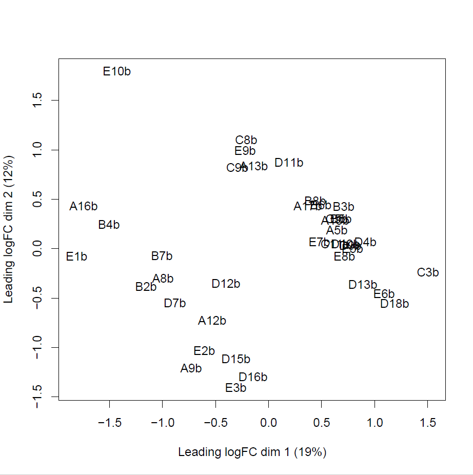
The cluster in the bottom left is female, and the cluster in the top right is male.
> X <- poly(Samples$Behavioral_Impulsivity, degree=3)
> design <- model.matrix(~X)
> design
(Intercept) X1 X2 X3
1 1 -0.0472438205 0.006707037 0.17317674
2 1 -0.0472438205 0.006707037 0.17317674
3 1 -0.0951011972 0.101004670 -0.07371293
4 1 -0.0951011972 0.101004670 -0.07371293
5 1 0.0006135561 -0.074459743 0.26311439
6 1 0.0006135561 -0.074459743 0.26311439
7 1 0.0963283094 -0.197400745 0.06411471
8 1 0.0963283094 -0.197400745 0.06411471
9 1 -0.0472438205 0.006707037 0.17317674
10 1 0.1441856861 -0.239174966 -0.17883209
11 1 0.0484709328 -0.142495670 0.21909529
12 1 0.1441856861 -0.239174966 -0.17883209
13 1 0.0484709328 -0.142495670 0.21909529
14 1 -0.0951011972 0.101004670 -0.07371293
15 1 0.0484709328 -0.142495670 0.21909529
16 1 -0.0472438205 0.006707037 0.17317674
17 1 -0.0951011972 0.101004670 -0.07371293
18 1 -0.0951011972 0.101004670 -0.07371293
19 1 -0.0951011972 0.101004670 -0.07371293
20 1 0.0125779003 -0.092699742 0.26376981
21 1 0.1441856861 -0.239174966 -0.17883209
22 1 0.0963283094 -0.197400745 0.06411471
23 1 -0.0951011972 0.101004670 -0.07371293
24 1 -0.0951011972 0.101004670 -0.07371293
25 1 -0.0951011972 0.101004670 -0.07371293
26 1 -0.0951011972 0.101004670 -0.07371293
27 1 0.8141889593 0.554725481 0.06081124
28 1 -0.0352794764 -0.014815676 0.20947715
29 1 0.1920430627 -0.267818335 -0.48674983
30 1 0.1441856861 -0.239174966 -0.17883209
31 1 -0.0951011972 0.101004670 -0.07371293
32 1 -0.0951011972 0.101004670 -0.07371293
33 1 -0.0951011972 0.101004670 -0.07371293
34 1 -0.0951011972 0.101004670 -0.07371293
35 1 -0.0951011972 0.101004670 -0.07371293
36 1 -0.0951011972 0.101004670 -0.07371293
37 1 -0.0951011972 0.101004670 -0.07371293
38 1 -0.0951011972 0.101004670 -0.07371293
39 1 -0.0951011972 0.101004670 -0.07371293
attr(,"assign")
[1] 0 1 1 1
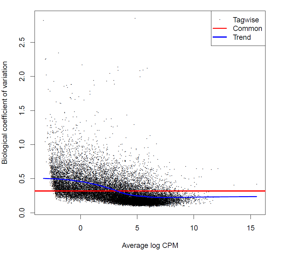
# estimate dispersion
> y <- estimateDisp(y, design)
> sqrt(y$common.dispersion)
[1] 0.3197842
#plot BCV
> plotBCV(y)
#use generalized linear model Quasi-likelihood F-Test

> fit <- glmQLFit(y, design, robust=TRUE)
> plotQLDisp(fit)
> fit <- glmQLFTest(fit, coef=2:4)

# Here are my significant genes

> tab <- as.data.frame(topTags(fit, n=50))
> tab
                logFC.X1    logFC.X2   logFC.X3       logCPM         F
C2CD4A        2.15801061 -2.04799644 -5.0737903 -0.570555005 33.294764
GTSF1         4.12537173  2.63843295 -0.2208206 -1.995873144 27.141999
FOSL1         1.53139823 -3.82697070 -5.0050511  0.113930746 23.689013
GRHL3         1.72382658 -2.87178251 -4.2065701 -1.593529596 20.953179
FAM183A      -3.35733234 -8.75949410  9.9841589 -0.338194308 20.326865
SFN           0.07403583 -3.06643783 -8.0580979  0.510316229 18.086643
LIF          -2.82915892 -4.62459485 -8.3351081 -0.544232368 15.275749
APOL4         0.81978733 -1.58355963 -2.5328564  0.953575299 14.812804
PZP          -0.63932534 -3.69184004  6.9933643  0.838428693 13.561366
CCDC42B       1.11605639 -3.60866135  6.3601651  0.804947539 12.960541
CCDC33       -0.49312788 -5.84549423  7.4114642 -0.220556512 12.865918
SLC5A7       -0.72455384 -9.23769807  6.7415073 -1.778769009 12.272693
CLCF1        -0.50545208 -1.63852222 -2.8779587  0.487658068 12.140901
SYNDIG1L      1.79295553 -3.66196801  6.0664507  3.697212708 11.856815
FAM216B       1.49774219 -3.59394497  8.5110450 -0.096603844 11.624245
DNAH3         1.96489905 -3.42699590  6.7111874  0.080493745 11.347664
TPMT          0.75677820  0.53259059 -0.2182363  5.519937269 11.220956
DNAH12       -0.03845676 -3.01513763  5.6722950  0.463394199 11.139964
SPAG17        1.95428708 -4.69638328  5.1351825  0.863309626 11.134328
CCDC37       -0.20605596 -3.45477922  5.5056977  1.261472648 11.107584
LPPR1         0.14941747 -1.09087064  1.4838642  3.791535285 10.959311
CHURC1        0.63500761  0.49930592  1.6207270  5.602509535 10.951865
HAS2          0.01865565 -2.32811262  1.5460027 -1.118283713 10.916301
STC1         -2.61572645 -2.52256129 -4.5848505 -0.092017347 10.902491
AGBL2        -0.25532620 -4.73328879  6.3275157  0.216973014 10.857938
CCL2          1.05563927 -0.01920003 -4.7557557  1.133151048 10.723222
C9orf117      1.27748816 -3.72184353  5.8279888  2.320872495 10.683779
MAP3K19       0.79913864 -3.19174199  7.2855162 -0.274451944 10.671556
GDNF-AS1     -0.40020458 -1.41688049  2.3415868  0.428643557 10.547675
IL1B          1.67146698 -1.25688950 -4.4060201  0.404654923 10.459701
ADAMTS9       0.42477076 -1.92583738 -1.8605483  2.504672213 10.188711
LOC101928817  2.36790748 -3.80383996  5.5877995 -0.693212168 10.106829
MT1A          0.82380492 -1.82102633 -3.9913299 -0.308825107 10.066389
ASB16        -0.93788882 -0.76250206  1.3699335 -0.037040670  9.821083
PLEKHH2      -0.59555404 -0.46742298  1.7042500  3.916933170  9.778554
HPYR1         0.61543358 -1.17376933 -2.8297364 -1.558557121  9.708399
MAP2K3       -0.20683496 -0.25349836 -1.4983857  3.781486607  9.694811
TEKT1        -0.09717566 -3.70370898  6.0523444  0.183338914  9.690371
C6orf118      0.37329086 -3.24204798  5.0081137 -0.287374231  9.622065
LRRC71        0.05143317 -5.48873866  6.6566840  0.006075004  9.571173
FAM81B        0.24674540 -4.27027257  5.5588747 -0.466371816  9.502256
LOC101928101 -4.70428068 -4.14538558 -2.1586718 -1.100670882  9.449353
ATP5E         0.99019435  1.09650967  0.5666700  4.108898617  9.442727
SLC7A5P1     -3.64861234 -0.80869921  1.7718580 -0.884600741  9.301228
LOC154761    -0.60501073  0.12179528 -1.8988382  1.096771561  9.294157
GLRX          0.09123528  0.68553310 -1.2470928  4.916519294  9.284804
IGFBP7-AS1    0.77205057 -3.97330198  4.7486815 -0.164360770  9.236343
LOC101929506 -3.59540113 -4.60320155  1.4959368 -2.118642940  9.118499
C9orf135      0.61491500 -2.33814430  5.8208234 -1.827029251  8.967774
EMP1         -1.46804817 -1.84162176 -4.8691728  3.911318859  8.945220
                   PValue          FDR
C2CD4A       7.880663e-11 1.630430e-06
GTSF1        1.227763e-09 1.270060e-05
FOSL1        6.917704e-09 4.770680e-05
GRHL3        3.060957e-08 1.583204e-04
FAM183A      5.139345e-08 2.126558e-04
SFN          1.658211e-07 5.717789e-04
LIF          1.014102e-06 2.997252e-03
APOL4        1.389372e-06 3.593090e-03
PZP          3.339753e-06 7.677350e-03
CCDC42B      5.161134e-06 1.040503e-02
CCDC33       5.532181e-06 1.040503e-02
SLC5A7       9.365424e-06 1.511018e-02
CLCF1        9.494533e-06 1.511018e-02
SYNDIG1L     1.178011e-05 1.740848e-02
FAM216B      1.407985e-05 1.941986e-02
DNAH3        1.744258e-05 2.121194e-02
TPMT         1.925556e-05 2.121194e-02
DNAH12       2.051723e-05 2.121194e-02
SPAG17       2.060819e-05 2.121194e-02
CCDC37       2.104565e-05 2.121194e-02
LPPR1        2.365444e-05 2.121194e-02
CHURC1       2.379408e-05 2.121194e-02
HAS2         2.447312e-05 2.121194e-02
STC1         2.474227e-05 2.121194e-02
AGBL2        2.563191e-05 2.121194e-02
CCL2         2.853218e-05 2.197032e-02
C9orf117     2.944504e-05 2.197032e-02
MAP3K19      2.973411e-05 2.197032e-02
GDNF-AS1     3.283775e-05 2.342690e-02
IL1B         3.524709e-05 2.430757e-02
ADAMTS9      4.390650e-05 2.930263e-02
LOC101928817 4.694205e-05 3.034950e-02
MT1A         4.852175e-05 3.042020e-02
ASB16        5.937990e-05 3.603198e-02
PLEKHH2      6.150838e-05 3.603198e-02
HPYR1        6.519616e-05 3.603198e-02
MAP2K3       6.593688e-05 3.603198e-02
TEKT1        6.618082e-05 3.603198e-02
C6orf118     7.005546e-05 3.716353e-02
LRRC71       7.309670e-05 3.780744e-02
FAM81B       7.743755e-05 3.907574e-02
LOC101928101 8.095286e-05 3.916709e-02
ATP5E        8.140486e-05 3.916709e-02
SLC7A5P1     9.171542e-05 4.182686e-02
LOC154761    9.226531e-05 4.182686e-02
GLRX         9.299800e-05 4.182686e-02
IGFBP7-AS1   9.689330e-05 4.265161e-02
LOC101929506 1.070972e-04 4.616114e-02
C9orf135     1.218174e-04 5.138996e-02
EMP1         1.241963e-04 5.138996e-02

> summary(decideTests(fit))
       X3-X2-X1
NotSig    20641
Sig          48
I ran a separate analysis without accounting for sex as a biological variable, and got 38 significant genes that were identical to this list. I inferred that the 10 additional significant genes were due to biological sex.
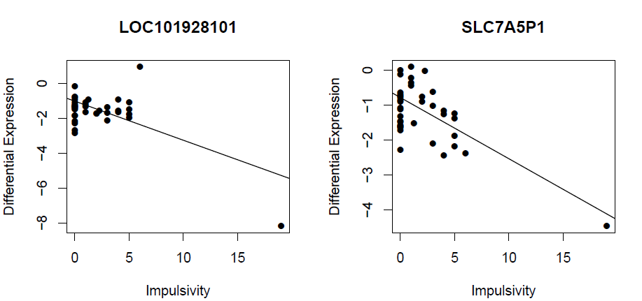
I'm also going to include a copy of the charts that I made in ggplot2
> logCPM.obs <- cpm(y, log=TRUE, prior.count=fit$prior.count)
> logCPM.fit <- cpm(fit, log=TRUE)

#Now we do the charts

> par(mfrow=c(2,2))
> for(i in 44:45) {
+ Gene <- row.names(tab)[i]
+ Symbol <- tab$Symbol[i]
+ logCPM.obs.i <- logCPM.obs[Gene, ]
+ logCPM.fit.i <- logCPM.fit[Gene, ]
+ plot(Samples$ImpulsivityScore, logCPM.obs.i, ylab="Differential Expression", xlab="Impulsivity", main=Gene, pch=16)
+ abline(lm(logCPM.fit.i ~ Samples$ImpulsivityScore))
+ }
Is my code examining what I say it is? If any more information is needed, please let me know.
Thank you for your help!