tl;dr: The most differentially expressed genes from DESeq2 are genes with very low read counts for many of my samples, and extremely high read counts for a few, even with pre-filtering - is this correct?

Hi!

I have a dataset comprising over 700 unique cell lines, each with a sensitivity data point (AUC) representing the response to a drug (measured by CellTiter-Glo assay). I have sourced a counts matrix with corresponding basal gene expression for matching cell lines with over 50,000 protein coding and non-protein coding genes here. I would like to see if sensitivity of my cell lines to my drug corresponds with differences in basal gene expression. e.g. high/increasing expression of protein x is significantly associated with sensitivity to my drug.

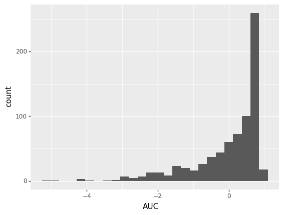
Here is a histogram of my AUC data:

I have created a DESeq Dataset as follows:

deseq_ds = DESeqDataSetFromMatrix(countData = round(counts),
                       colData = viab,
                       design = ~ AUC)
`

Where viab is a cell line identifier as rowname and single column containing centered and scaled AUC values.

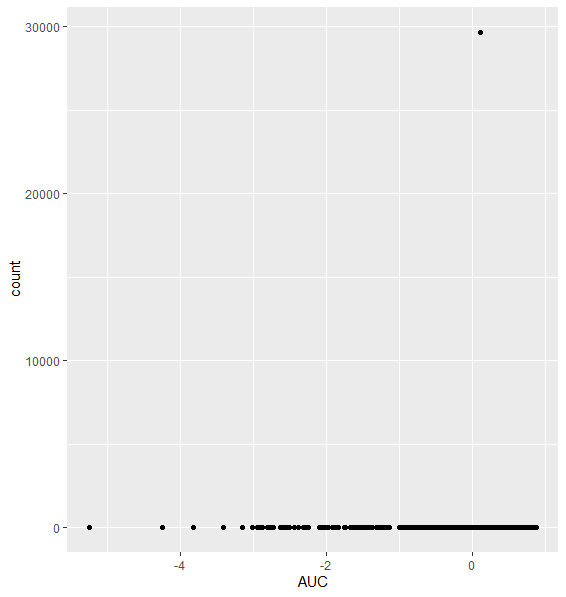
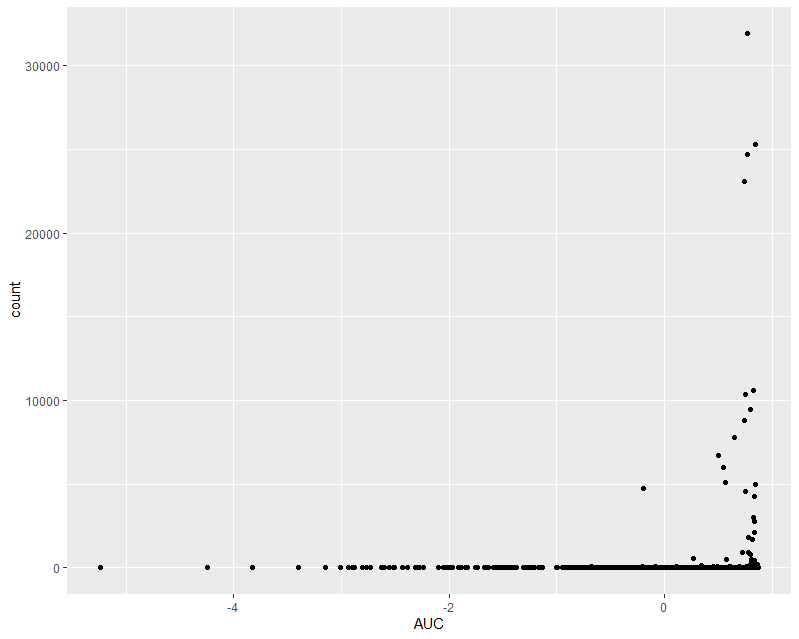
I started to run into issues (I think?!) when I was running the code without pre-filtering, and plotting counts of my most significantly differentially expressed genes (ordered by adjusted p-value):

plt = plotCounts(deseq_ds, gene=idx, intgroup = 'AUC', returnData = T)
## plot with ggplot

As you can see, we have one extreme outlier gene that is seemingly producing this significance. I added pre-filtering to exclude this, by filtering out genes with <= 10 samples with counts <= 50.

  keep = rowSums(counts(deseq_ds) >= 10) >= 50
  deseq_ds = deseq_ds[keep,]

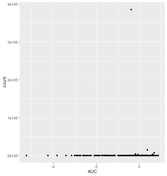
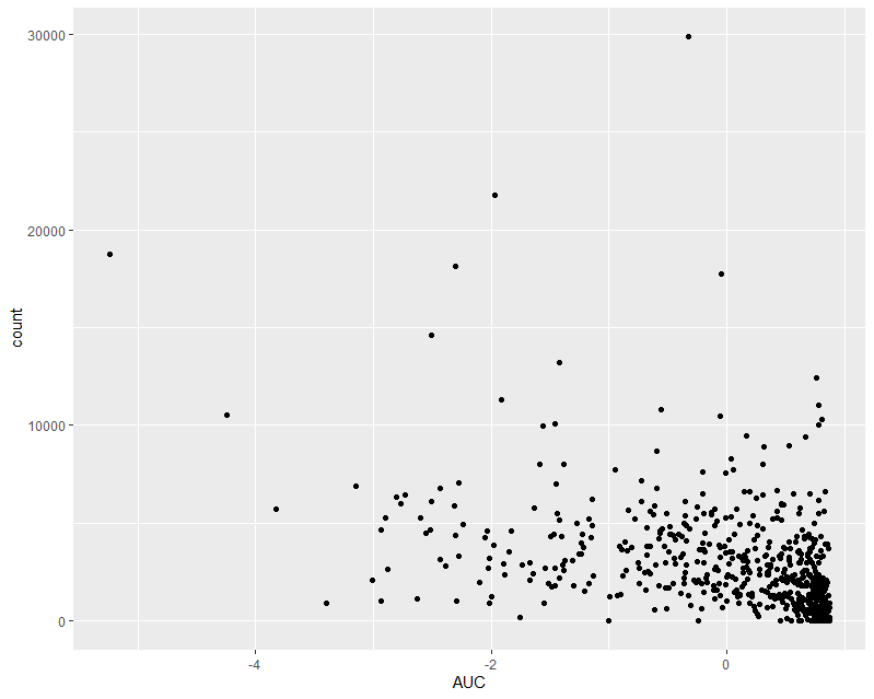
I replotted the most significant gene (padj 6.87e-73) (this gene also has one of the highest absolute LFC (-2.979)):

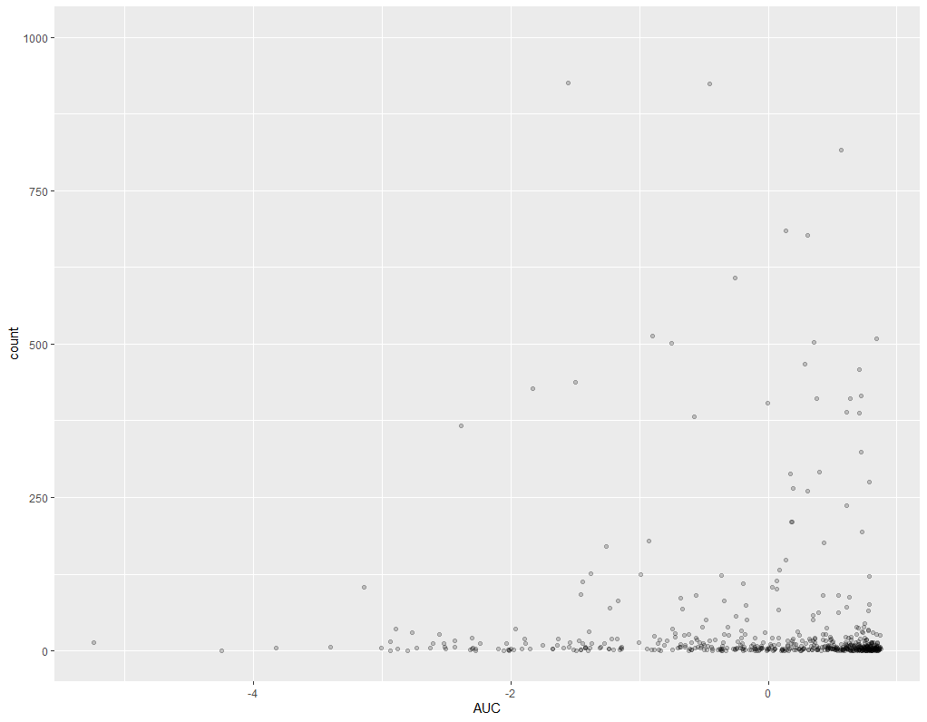
Adding ylim 0 -> 1000 to zoom into interesting part:

Here is another example, with 3rd most significant gene, (padj 3.51e-47, log2FC 2.79):

Here is an example where I feel a trend is more noticeable, and the results seem more realistic (padj 1.7e-15; log2FC -0.47):

I am a bit confused, as pretty much all of the most significant plots don't look very convincing and from visual inspection I don't think I would say there is even a trend based on this data. They seem to being heavily skewed by a few samples with extremely high read count.

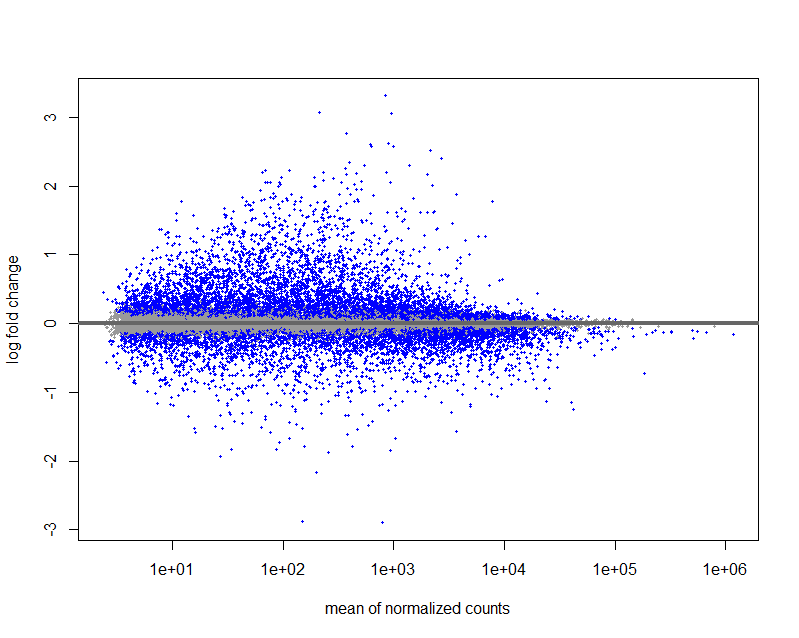
Furthermore, I have >9000 genes significant in my dataset, of a total of 26433 (following pre-filtering) which is approximately 1/3 of all my genes are being classified as DEGs. Is this quite high?

Am I doing something wrong here or making an assumption I shouldn't be? Is DESeq2 suited to this kind of analysis, or should I be using a different package? Or does everything look like it's working as intended? Thanks for any help and guidance!

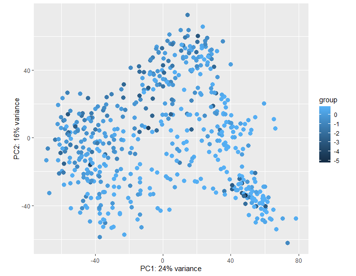
Here is my PCA plot:

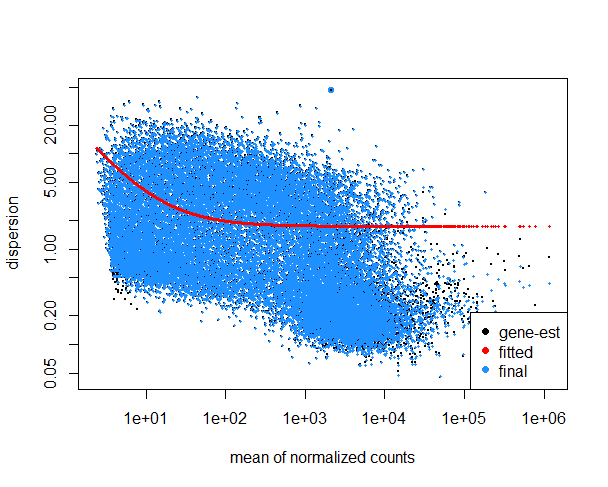
Here is plot of my gene dispersion (it's very high, I believe?):

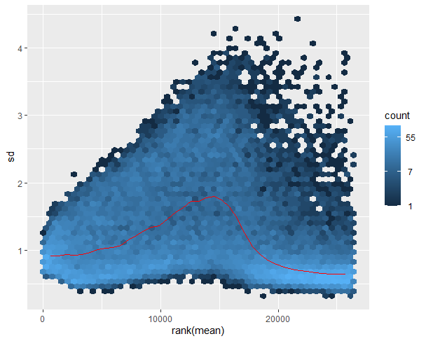
Here is plot of my SD against ranked mean following VTS normalisation:

Here is my MA plot: