Hello, I am running differential expression analysis on age-related changes in transcription using natural splines with DESeq2 like so:

    dds <- DESeqDataSetFromMatrix(countData = counts,
                                  colData = coldata,
                                 design = ~ ns(age_scaled, df = 3))

keep <- rowSums(counts(dds) >= 10) >= 3
dds <- dds[keep,]


dds <- DESeq(dds, test="LRT", reduced = ~ 1)
res <- results(dds)

And later plotting the fitted splines like so:

# Matrices for fitted curves:
coef_mat <- coef(dds)
design_mat <- model.matrix(design(dds), colData(dds))


dat <- plotCounts(dds, gene, intgroup = c("age", "sex", "genotype"), returnData = TRUE) %>%
    mutate(logmu = design_mat %*% coef_mat[gene,],
           logcount = log2(count + 1))

ggplot(dat, aes(age, logcount)) +
    geom_point(aes(color = age, shape = genotype), size = 2) +
    geom_line(aes(age, logmu), col="#FF7F00", linewidth = 1.2) +
    labs(
      title = gene, 
      x = "Age", 
      y = "Log2 expression count", 
      color = "Age"
    )

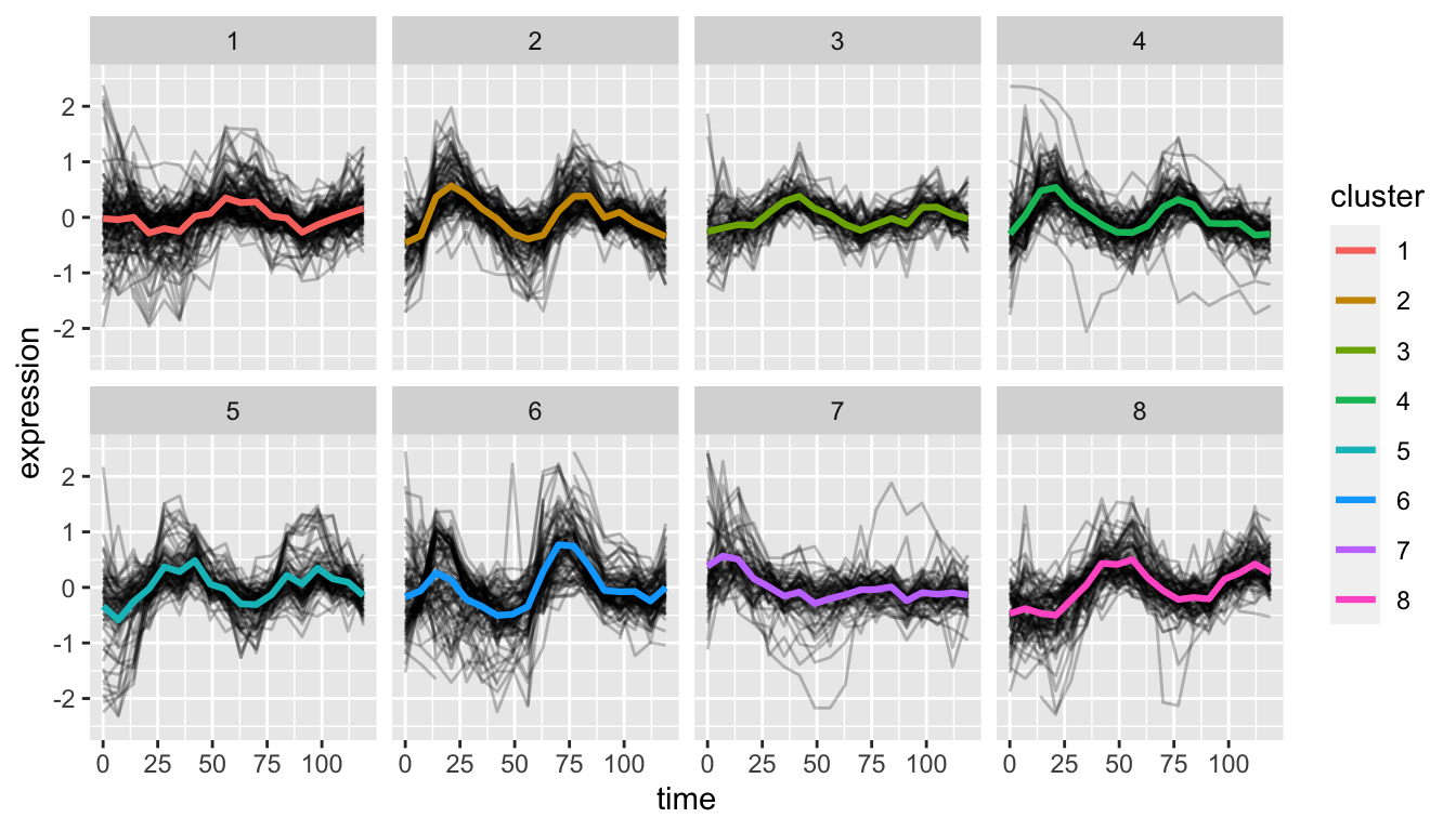
I clustered the genes with kmeans and now apart from profiling the clusters I would like to visualize them, similar to an approach here: from: https://bio723-class.github.io/Bio723-book/clustering-in-r.html#depicting-the-data-within-clusters

But in my case I do not have per group LFC as I was doing LRT. Any advice/ideas if I could still do a similar vizualization; extracting the splines per gene in my gene_list and perhaps putting Z-scores on the y-axis? I am struggling to figure out a way to reapply the code to my data. Thanks a lot in advance.

sessionInfo( )
R version 4.3.1 (2023-06-16 ucrt)
Platform: x86_64-w64-mingw32/x64 (64-bit)
Running under: Windows 11 x64 (build 22621)

Matrix products: default


locale:
[1] LC_COLLATE=English_United States.utf8  LC_CTYPE=English_United States.utf8   
[3] LC_MONETARY=English_United States.utf8 LC_NUMERIC=C                          
[5] LC_TIME=English_United States.utf8    

time zone: Europe/Berlin
tzcode source: internal

attached base packages:
[1] splines   stats4    stats     graphics  grDevices utils     datasets  methods   base     

other attached packages:
 [1] gplots_3.1.3                cluster_2.1.4               dendextend_1.17.1          
 [4] umap_0.2.10.0               vsn_3.68.0                  shiny_1.7.5                
 [7] xlsx_0.6.5                  readxl_1.4.3                EnhancedVolcano_1.18.0     
[10] ggrepel_0.9.3               RColorBrewer_1.1-3          pheatmap_1.0.12            
[13] DESeq2_1.40.2               SummarizedExperiment_1.30.2 Biobase_2.60.0             
[16] MatrixGenerics_1.12.3       matrixStats_1.0.0           GenomicRanges_1.52.0       
[19] GenomeInfoDb_1.36.1         IRanges_2.34.1              S4Vectors_0.38.1           
[22] BiocGenerics_0.46.0         lubridate_1.9.2             forcats_1.0.0              
[25] stringr_1.5.0               dplyr_1.1.2                 purrr_1.0.2                
[28] readr_2.1.4                 tidyr_1.3.0                 tibble_3.2.1               
[31] ggplot2_3.4.3               tidyverse_2.0.0             BiocManager_1.30.22        

loaded via a namespace (and not attached):
 [1] bitops_1.0-7            gridExtra_2.3           rlang_1.1.1             magrittr_2.0.3         
 [5] compiler_4.3.1          png_0.1-8               systemfonts_1.0.5       vctrs_0.6.3            
 [9] pkgconfig_2.0.3         crayon_1.5.2            fastmap_1.1.1           XVector_0.40.0         
[13] ellipsis_0.3.2          labeling_0.4.3          caTools_1.18.2          utf8_1.2.3             
[17] promises_1.2.1          rmarkdown_2.25          tzdb_0.4.0              preprocessCore_1.62.1  
[21] ragg_1.2.6              bit_4.0.5               xfun_0.40               zlibbioc_1.46.0        
[25] cachem_1.0.8            jsonlite_1.8.7          later_1.3.1             DelayedArray_0.26.7    
[29] xlsxjars_0.6.1          BiocParallel_1.34.2     parallel_4.3.1          R6_2.5.1               
[33] bslib_0.5.1             stringi_1.7.12          reticulate_1.34.0       limma_3.56.2           
[37] jquerylib_0.1.4         cellranger_1.1.0        Rcpp_1.0.11             knitr_1.44             
[41] httpuv_1.6.11           Matrix_1.5-4.1          timechange_0.2.0        tidyselect_1.2.0       
[45] viridis_0.6.4           rstudioapi_0.15.0       abind_1.4-5             yaml_2.3.7             
[49] codetools_0.2-19        affy_1.78.2             curl_5.0.2              lattice_0.21-8         
[53] withr_2.5.1             askpass_1.2.0           evaluate_0.22           rJava_1.0-6            
[57] pillar_1.9.0            affyio_1.70.0           KernSmooth_2.23-21      generics_0.1.3         
[61] vroom_1.6.4             RCurl_1.98-1.12         hms_1.1.3               munsell_0.5.0          
[65] scales_1.2.1            gtools_3.9.4            xtable_1.8-4            glue_1.6.2             
[69] tools_4.3.1             hexbin_1.28.3           RSpectra_0.16-1         locfit_1.5-9.8         
[73] grid_4.3.1              colorspace_2.1-0        GenomeInfoDbData_1.2.10 cli_3.6.1              
[77] textshaping_0.3.7       fansi_1.0.4             viridisLite_0.4.2       S4Arrays_1.0.5         
[81] gtable_0.3.4            sass_0.4.7              digest_0.6.33           farver_2.1.1           
[85] htmltools_0.5.6         lifecycle_1.0.3         mime_0.12               bit64_4.0.5            
[89] openssl_2.1.1