Question

Microarray Limma Model fitting and DEG

0

Entering edit mode

Amit • 0

@b648b3f5

Last seen 9 days ago

India

Hi, Why I am not getting Up and Down regulated genes? My script is as below m I missed something or doing wrong ?

getGEOSuppFiles("GSE18090")

Untar and ReadAffy(rawdata).

gse <- getGEO("GSE18090", GSEMatrix = TRUE)

extracting phenodata and desired column from it as (phenodata$groups).

#Normalization
normdata <- rma(rawdata)
normexprs <- exprs(normdata)

#Limma
design <- model.matrix(~0+phenodata$groups)
colnames(design) <- c("NRM","SVR","CTL")
fit <- lmFit(normexprs, design)
contrasts <- makeContrasts(CTL-NRM, CTL-SVR, NRM-CTL, levels=design)
fit2 <- contrasts.fit(fit, contrasts)
fit2 <- eBayes(fit2)
topTable(fit2)
  0 
164025
decideTests(fit2)
table(decideTests(fit2))
Results <- decideTests(fit2)
summary(Results)
     CTL-NRM CTL-SVR NRM-CTL
Down         0        0        0
NotSig   54675    54675    54675
Up           0        0        0

limma DGEanalysis • 504 views

ADD COMMENT • link updated 4 weeks ago by Gordon Smyth 50k • written 4 weeks ago by Amit • 0

score 1 · Answer 1 · 2024-03-26

1

Entering edit mode

James W. MacDonald 65k

@james-w-macdonald-5106

Last seen 15 hours ago

United States

The short answer is because there is no evidence for any differences. A longer answer is to say that you haven't included enough information for anybody to repeat what you have done, so it's not possible for anybody to say anything more than the short answer.

ADD COMMENT • link 4 weeks ago James W. MacDonald 65k

0

Entering edit mode

> print(PHENO)
                Patients Group
GSM452235   DF Patient 1    DF
GSM452236   DF Patient 2    DF
GSM452237   DF Patient 3    DF
GSM452238   DF Patient 4    DF
GSM452239   DF Patient 5    DF
GSM452240   DF Patient 6    DF
GSM452241   DF Patient 7    DF
GSM452242   DF Patient 8    DF
GSM452243  DHF Patient 1   DHF
GSM452244  DHF Patient 2   DHF
GSM452245  DHF Patient 3   DHF
GSM452246  DHF Patient 4   DHF
GSM452247  DHF Patient 5   DHF
GSM452248  DHF Patient 6   DHF
GSM452249  DHF Patient 7   DHF
GSM452250  DHF Patient 8   DHF
GSM452251  DHF Patient 9   DHF
GSM452252 DHF Patient 10   DHF
GSM452253   ND Patient 1    ND
GSM452254   ND Patient 2    ND
GSM452255   ND Patient 3    ND
GSM452256   ND Patient 4    ND
GSM452257   ND Patient 5    ND
GSM452258   ND Patient 6    ND
GSM452259   ND Patient 7    ND
GSM452260   ND Patient 8    ND
> NORM.data <-affy::rma(RAW.data)
Background correcting
Normalizing
Calculating Expression
> NORM.expr <- exprs(NORM.data)
> PHENO$Group
 [1] "DF"  "DF"  "DF"  "DF"  "DF"  "DF"  "DF"  "DF"  "DHF" "DHF" "DHF" "DHF" "DHF" "DHF" "DHF" "DHF" "DHF"
[18] "DHF" "ND"  "ND"  "ND"  "ND"  "ND"  "ND"  "ND"  "ND" 
> design <- model.matrix(~0+PHENO$Group)
> design
   PHENO$GroupDF PHENO$GroupDHF PHENO$GroupND
1              1              0             0
2              1              0             0
3              1              0             0
4              1              0             0
5              1              0             0
6              1              0             0
7              1              0             0
8              1              0             0
9              0              1             0
10             0              1             0
11             0              1             0
12             0              1             0
13             0              1             0
14             0              1             0
15             0              1             0
16             0              1             0
17             0              1             0
18             0              1             0
19             0              0             1
20             0              0             1
21             0              0             1
22             0              0             1
23             0              0             1
24             0              0             1
25             0              0             1
26             0              0             1
attr(,"assign")
[1] 1 1 1
attr(,"contrasts")
attr(,"contrasts")$`PHENO$Group`
[1] "contr.treatment"

> colnames(design) <- c("DF","DHF","ND")
> design
   DF DHF ND
1   1   0  0
2   1   0  0
3   1   0  0
4   1   0  0
5   1   0  0
6   1   0  0
7   1   0  0
8   1   0  0
9   0   1  0
10  0   1  0
11  0   1  0
12  0   1  0
13  0   1  0
14  0   1  0
15  0   1  0
16  0   1  0
17  0   1  0
18  0   1  0
19  0   0  1
20  0   0  1
21  0   0  1
22  0   0  1
23  0   0  1
24  0   0  1
25  0   0  1
26  0   0  1
attr(,"assign")
[1] 1 1 1
attr(,"contrasts")
attr(,"contrasts")$`PHENO$Group`
[1] "contr.treatment"

> fit <- lmFit(NORM.expr, design)
> head(fit$coefficients)
                DF      DHF       ND
1007_s_at 6.765789 6.629171 6.912516
1053_at   7.138876 7.291011 6.868875
117_at    7.526406 7.112309 6.737322
121_at    8.604059 8.446119 8.539832
1255_g_at 3.475019 3.507082 3.507321
1294_at   9.975198 9.676852 9.775188
> contrasts <- makeContrasts(ND - DF, ND - DHF, DF - DHF, levels=design)
> fit2 <- contrasts.fit(fit, contrasts)
> fit2 <- eBayes(fit2)
> topTable(fit2)
                ND...DF   ND...DHF    DF...DHF   AveExpr        F      P.Value adj.P.Val
236191_at   -1.76082176 -2.0129321 -0.25211032  8.758478 19.42771 7.613311e-06 0.2718143
226959_at    0.78600129  0.8255397  0.03953838  7.889951 18.07446 1.314852e-05 0.2718143
229114_at   -0.26045076 -1.2031619 -0.94271116  5.807734 17.72116 1.522476e-05 0.2718143
228910_at    0.41791523  0.4826820  0.06476680  7.190302 16.92195 2.134805e-05 0.2718143
224806_at   -1.50548644 -1.0934605  0.41202590 11.361303 15.43618 4.103245e-05 0.2718143
219283_at   -0.89278828 -1.4547205 -0.56193219  8.278945 15.21822 4.529111e-05 0.2718143
232884_s_at  0.44806045  0.5228403  0.07477984  4.841676 15.04643 4.898361e-05 0.2718143
226876_at    0.97043591  0.9193631 -0.05107278  9.637218 14.95229 5.114371e-05 0.2718143
226002_at    0.03453007 -0.5374355 -0.57196554  4.643638 14.88797 5.267849e-05 0.2718143
212300_at   -0.91891702 -0.5848127  0.33410433  7.064833 14.76720 5.569641e-05 0.2718143
> decideTests(fit2)
TestResults matrix
           Contrasts
            ND - DF ND - DHF DF - DHF
  1007_s_at       0        0        0
  1053_at         0        0        0
  117_at          0        0        0
  121_at          0        0        0
  1255_g_at       0        0        0
54670 more rows ...
> table(decideTests(fit2))

     0 
164025 
> Results <- decideTests(fit2)
> summary(Results)
       ND - DF ND - DHF DF - DHF
Down         0        0        0
NotSig   54675    54675    54675
Up           0        0        0
>

ADD REPLY • link 4 weeks ago Amit • 0

0

Entering edit mode

Hi James, Sorry for mistake.

ADD REPLY • link 4 weeks ago Amit • 0

0

Entering edit mode

The original paper used individual t-tests, and apparently did not adjust for multiple comparisons. That's not how it's done. In addition, with a t-test you ignore sex-specific differences which is problematic as well. Ideally you would do something like this.

> library(affycoretools)
> library(hgu133plus2.db)
> eset <- rma(ReadAffy())
> eset <- annotateEset(eset, hgu133plus2.db)
> pd <- pData(gse[[1]])
> d.f <- data.frame(Age = as.numeric(as.character(pd[,44])), Sex = pd[,46], Status = factor(rep(c("DF","DHF","ND"), c(8,10,8)), c("ND","DF","DHF")))
> d.f
   Age    Sex Status
1   30 female     DF
2   40 female     DF
3   45   male     DF
4   53   male     DF
5   29 female     DF
6   27   male     DF
7   44   male     DF
8   23 female     DF
9   41   male    DHF
10  41 female    DHF
11  84 female    DHF
12  26 female    DHF
13  19   male    DHF
14  22 female    DHF
15  36   male    DHF
16  35 female    DHF
17  21 female    DHF
18  21 female    DHF
19  41   male     ND
20  25   male     ND
21  47   male     ND
22  54   male     ND
23  23 female     ND
24  19 female     ND
25  30 female     ND
26  64 female     ND
> design <- model.matrix(~0 + Status + Sex, d.f)
> colnames(design) <- gsub("Status","", colnames(design))
> contrast <- makeContrasts(DF - ND, DHF - ND, DHF - DF, levels = design)
> fit <- eBayes(contrasts.fit(lmFit(eset, design), contrast))
> summary(decideTests(fit))
       DF - ND DHF - ND DHF - DF
Down         0        0        0
NotSig   54675    54675    54675
Up           0        0        0
> lapply(1:3, function(x) topTable(fit, x, 3))
[[1]]
                PROBEID  ENTREZID
224806_at     224806_at      7706
212300_at     212300_at    200081
210212_x_at 210212_x_at 100272147
            SYMBOL
224806_at   TRIM25
212300_at    TXLNA
210212_x_at   CMC4
                                  GENENAME
224806_at   tripartite motif containing 25
212300_at                    taxilin alpha
210212_x_at      C-X9-C motif containing 4
                 logFC   AveExpr
224806_at    1.5054864 11.361303
212300_at    0.9189170  7.064833
210212_x_at -0.7079183  7.261891
                    t      P.Value
224806_at    5.500865 1.108939e-05
212300_at    5.287946 1.902779e-05
210212_x_at -5.233557 2.185178e-05
            adj.P.Val        B
224806_at   0.3695115 1.569699
212300_at   0.3695115 1.251449
210212_x_at 0.3695115 1.169082

[[2]]
            PROBEID ENTREZID SYMBOL
229114_at 229114_at     2549   GAB1
236191_at 236191_at     <NA>   <NA>
228910_at 228910_at     3732   CD82
                                   GENENAME
229114_at GRB2 associated binding protein 1
236191_at                              <NA>
228910_at                     CD82 molecule
               logFC  AveExpr
229114_at  1.2597600 5.807734
236191_at  2.0333548 8.758478
228910_at -0.5019084 7.190302
                  t      P.Value
229114_at  5.915460 3.914680e-06
236191_at  5.747672 5.955761e-06
228910_at -5.705006 6.629060e-06
          adj.P.Val        B
229114_at 0.1208146 3.850087
236191_at 0.1208146 3.513941
228910_at 0.1208146 3.427843

[[3]]
                PROBEID ENTREZID
226002_at     226002_at     2549
229114_at     229114_at     2549
220177_s_at 220177_s_at    64699
             SYMBOL
226002_at      GAB1
229114_at      GAB1
220177_s_at TMPRSS3
                                     GENENAME
226002_at   GRB2 associated binding protein 1
229114_at   GRB2 associated binding protein 1
220177_s_at   transmembrane serine protease 3
                 logFC  AveExpr
226002_at    0.5883623 4.643638
229114_at    0.9993092 5.807734
220177_s_at -0.9616712 5.018456
                    t      P.Value
226002_at    4.806629 6.506156e-05
229114_at    4.692461 8.718634e-05
220177_s_at -4.659076 9.498060e-05
            adj.P.Val         B
226002_at   0.9999349 -1.809867
229114_at   0.9999349 -1.895525
220177_s_at 0.9999349 -1.920819

Which provides no evidence for any differential expression. You could try array weights, which helps somewhat, as does relaxing to a 10% FDR

> wts <- arrayWeights(eset, design)
> fit <- eBayes(contrasts.fit(lmFit(eset, design, weights = wts), contrast))
> summary(decideTests(fit))
       DF - ND DHF - ND DHF - DF
Down         0        0        0
NotSig   54674    54675    54675
Up           1        0        0

> summary(decideTests(fit, p.value = 0.1))
       DF - ND DHF - ND DHF - DF
Down         9      141        0
NotSig   54661    54445    54675
Up           5       89        0

ADD REPLY • link 4 weeks ago James W. MacDonald 65k

score 1 · Answer 2 · 2024-03-27

This dataset seems straightforward to analyse using the original MAS expression values on GEO. MAS expression values are known to be noisy for low-intensity probe-sets but the limma-trend method handles that. Here is a reproducible analysis.

> library(GEOquery)
> gse <- getGEO("GSE18090", GSEMatrix = TRUE)
Found 1 file(s)
GSE18090_series_matrix.txt.gz
> gse <- gse[[1]]
> y <- log2(exprs(gse))
> Disease <- rep(c("DF","DHF","ND"),c(8,10,8))
> Disease <- factor(Disease,levels=c("ND","DF","DHF"))
> Sex <- factor(pData(gse)$gender)
> Sample <- pData(gse)$title
> Sample <- sub(" Patient ","",Sample)
> colnames(y) <- Sample

> library(limma)
> design <- model.matrix(~Disease+Sex)
> fit <- lmFit(y,design)
> plotSA(fit)
> keep <- rowMeans(y) > 4
> yfilt <- y[keep,]
> w <- arrayWeights(yfilt,design)
> fit <- lmFit(yfilt,design,weights=w)
> fit <- eBayes(fit,trend=TRUE,robust=TRUE)
> plotSA(fit)
> summary(decideTests(fit))
       (Intercept) DiseaseDF DiseaseDHF Sexmale
Down             0         1        169       9
NotSig           0     32626      32033   32604
Up           32630         3        428      17

I have used array weights for this analysis because one of the samples appears to be an outlier. The use of array weights reduces the number of DE genes for DHF vs ND but makes me more confident in the results.

score 0 · Answer 3 · 2024-03-26

0

Entering edit mode

Gordon Smyth 50k

@gordon-smyth

Last seen 1 hour ago

WEHI, Melbourne, Australia

There was no evidence of any significant differences in the original PLOS ONE publication associated with this data. None of the p-values shown in the paper would remain significant after adjustment for multiple testing. So the lack of significant results is the same as in the original paper.

ADD COMMENT • link 4 weeks ago Gordon Smyth 50k

0

Entering edit mode

Hi Gordon and James,

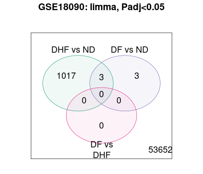
But NCBI GEO2R analysis (https://www.ncbi.nlm.nih.gov/geo/geo2r/?acc=GSE18090) shows reasonable results. Why it is so ? If the data is same then why wouldn't we get results ? Is Raw data and Series Matrix data gives us different results? Could you please look through it?

ADD REPLY • link 4 weeks ago Amit • 0

0

Entering edit mode

Taking into account only the status, the results look similar in the sense that the main difference is DHF vs ND, and most of the advertised genes relate to the Ig family.

enter image description here

ADD REPLY • link 4 weeks ago SamGG ▴ 350