Hi,
I'm trying to better grasp what is happening under the hood during dispersion estimation, and have a bit of a naive question. When using the makeExampleDESeqDataSet function, I can set the dispersions to zero by just specifying a 'null function', i.e.:
dds_pois <- makeExampleDESeqDataSet(
  n=5000,
  m=10,
  dispMeanRel = function(x) 0
)
and indeed the dispersions here are all zero, and thus our counts should follow Poisson (mean == var).
mcols(dds_pois) %>% head()

DataFrame with 6 rows and 3 columns
      trueIntercept  trueBeta  trueDisp
          <numeric> <numeric> <numeric>
gene1      5.016721         0         0
gene2      0.226108         0         0
.....
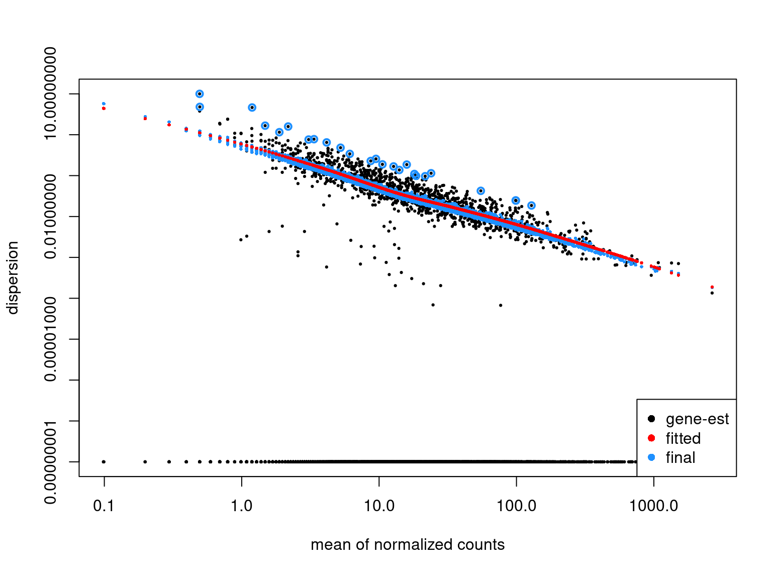
If I now run DESeq and plot the estimated dispersion:
dds_pois <- DESeq(dds_pois)
estimating size factors
estimating dispersions
gene-wise dispersion estimates
mean-dispersion relationship
-- note: fitType='parametric', but the dispersion trend was not well captured by the
   function: y = a/x + b, and a local regression fit was automatically substituted.
   specify fitType='local' or 'mean' to avoid this message next time.
final dispersion estimates
fitting model and testing
plotDispEsts(dds_pois, CV=TRUE)
I see a negative linear relationship between the counts and the estimated dispersion. I would expect the estimates to be a) all very close to the minimum (i.e. 1e-8) and b) not have any specific trend at all to begin with. Am I missing something in my interpretation ?
Thanks !


Thank you for the pointers, I'll revert back again to the method section of the paper. As for the negative relationship of the estimated dispersions, is it correct to assume that this is a result of the assumed mean-dependent prior for the dispersions (i.e. the alpha_tr in the manuscript) ?
The red line does assume that shape but the fact the black points show that pattern is discussed in the 2014 paper.