
Hi,
I've asked this in Biostars but I've been told I might have better luck here. I'll copy my question below:
(I'm currently editing the post to paste it because the editors is giving me trouble during the first posting)
I have a bulk RNA dataset. Mouse data. 2 genetic backgrounds (WT and mutant(Dmin)) which are a model of human disease. For each background I have:
- Young Control (6wk, AL)
- Adult Control (22wk, AL)
- Adult Treatment (22wk, DR)
4-5 samples each.
Although this data comes from a single sequencing experiment, the analysis was split into 2 papers led by different people (there is a lot of additional wet lab work on each of them, the RNA-seq is just a fraction of the analyses). Because of this, the first analysis was done using only the Young vs Adult (Control) samples (excluding Adult Treated samples from the DESeq2 object to prevent their interference and keep a balanced Young/Adult ratio) and has already been published.
The second analysis focuses on the Treatment part in Adults, but builds up on the results from the first analysis. It was decided that, similarly to what was done on the first analysis, here we would exclude the Young samples, and limit the DESeq2 object to only the Adult ones (both Treated and Control). However, an important part of the analysis focuses on comparing the DEG that changed in Mutant mice as they grew older (data generated ignoring adult+treatment mice), and how the treatment in adults affects some of those genes (data generated ignoring young mice). You can see where I'm going...
I have a couple of very interesting biologically relevant genes. If I analyze the data using all the samples (from now on deemed "ALL") both are significant. If I analyze the data using only the adult samples (now deemed "ADULT"), both genes have padj = NA. I am focusing mostly in the comparison 22DminDR vs 22DminAL (Adult Mutant samples, Treated vs Control)
This is how the normalized counts look like:
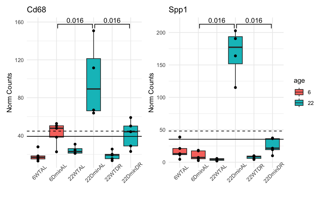
The dashed line is the baseMean in ADULT. The solid line is in ALL. The color of the boxplots is the sample's age. the ADULT analysis uses only the blue ones. The groups are significant when using a naive and simple T-test.
And these are the results of DESeq2 for the 22DminDR vs 22DminAL comparison:
ALL samples:
> res_all[c("Spp1","Cd68"),]
log2 fold change (MAP): modelvar 22DminDR vs 22DminAL
Wald test p-value: modelvar 22DminDR vs 22DminAL
DataFrame with 2 rows and 5 columns
      baseMean log2FoldChange     lfcSE      pvalue        padj
     <numeric>      <numeric> <numeric>   <numeric>   <numeric>
Spp1   35.4312       -2.72427  0.473436 2.76300e-10 1.79236e-06
Cd68   39.0621       -1.08386  0.320647 2.81564e-05 4.35931e-03
ADULT samples:
> res_adult[c("Spp1","Cd68"),]
log2 fold change (MAP): modelvar 22DminDR vs 22DminAL
Wald test p-value: modelvar 22DminDR vs 22DminAL
DataFrame with 2 rows and 5 columns
      baseMean log2FoldChange     lfcSE      pvalue      padj
     <numeric>      <numeric> <numeric>   <numeric> <numeric>
Spp1   48.1062       -2.80547  0.336887 1.39669e-18        NA
Cd68   44.6694       -1.03332  0.305645 2.64104e-05        NA
I have been reading about this from several sources:
https://bioconductor.org/packages/release/bioc/vignettes/DESeq2/inst/doc/DESeq2.html#pvaluesNA
Note on p-values set to NA: some values in the results table can be set to NA for one of the following reasons:
- If within a row, all samples have zero counts, the baseMean column will be zero, and the log2 fold change estimates, p value and adjusted p value will all be set to NA.
- If a row contains a sample with an extreme count outlier then the p value and adjusted p value will be set to NA. These outlier counts are detected by Cook's distance. Customization of this outlier filtering and description of functionality for replacement of outlier counts and refitting is described below
- If a row is filtered by automatic independent filtering, for having a low mean normalized count, then only the adjusted p value will be set to NA. Description and customization of independent filtering is described below
And following a few links,
https://bioconductor.org/packages/devel/bioc/vignettes/DESeq2/inst/doc/DESeq2.html#indfilt
https://bioconductor.org/packages/devel/bioc/vignettes/DESeq2/inst/doc/DESeq2.html#indfilttheory
DESeq2 cooksCutoff ON/OFF: pairwise contrasts for many groups, some with only 2 reps
I have been checking all these values for both comparisons:
- Cooks distance:
ADULT samples:
Control (Adult, Mutant)
> assays(dds_adult)[["cooks"]][c("Spp1","Cd68"), md[md$modelvar=="22DminAL",]$sample]
            005        013          004         026
Spp1 0.16294652 0.08470974 5.871258e-01 0.003260566
Cd68 0.09220205 0.03160875 6.519192e-05 0.025208679
Treatment (Adult, Mutant)
> assays(dds_adult)[["cooks"]][c("Spp1","Cd68"), md[md$modelvar=="22DminDR",]$sample]
             006          014        029        016          022
Spp1 0.097962191 0.0001170788 0.03350797 0.11415755 0.3792535252
Cd68 0.008037438 0.0421175078 0.04893443 0.08676744 0.0006556893
ALL samples:
Control (Adult, Mutant)
 > assays(dds_all)[["cooks"]][c("Spp1","Cd68"), md[md$modelvar=="22DminAL",]$sample]
            005        013         004         026
Spp1 0.05697454 0.04023993 0.250256327 0.002499021
Cd68 0.06793757 0.02701774 0.001844374 0.023258608
Treatment (Adult, Mutant)
> assays(dds_all)[["cooks"]][c("Spp1","Cd68"), md[md$modelvar=="22DminDR",]$sample]
             006          014        029        016         022
Spp1 0.052105796 1.310099e-05 0.02087917 0.06202494 0.165106367
Cd68 0.001446295 1.449497e-02 0.03282256 0.03355575 0.005948603
I don't think the cooks distance differences are large enough to justify removing these genes from the analysis
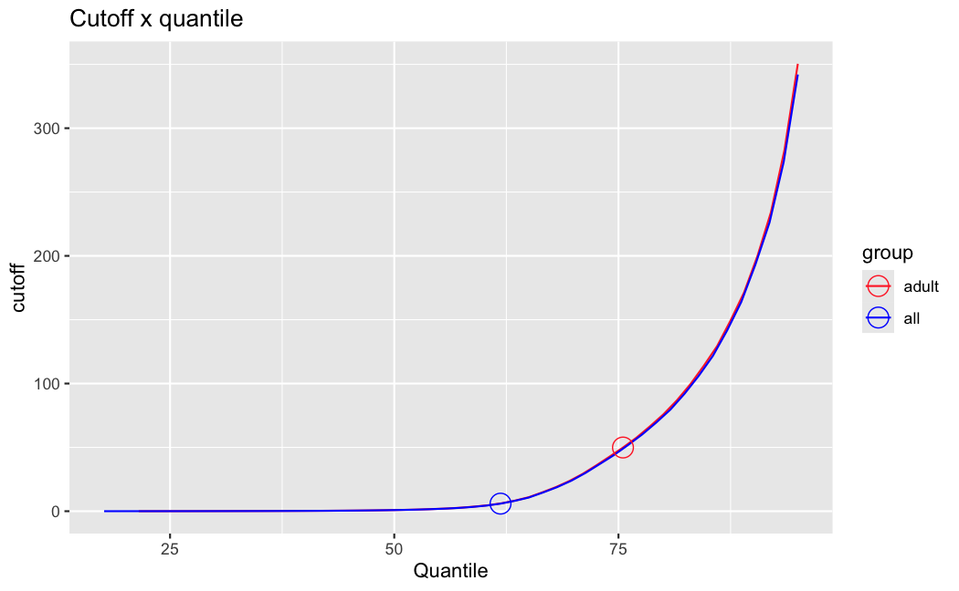
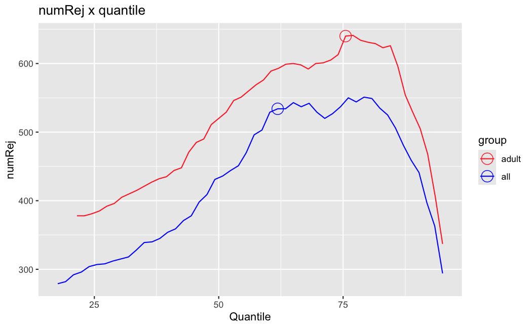
- Independent Filtering
Number of rejections: (ADULT vs ALL)
plot(metadata(res_all)$filterNumRej,
     type="b", ylab="number of rejections",
     xlab="quantiles of filter", main="ALL")
lines(metadata(res_all)$lo.fit, col="red")
abline(v=metadata(res_all)$filterTheta)
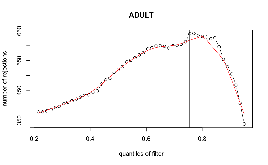
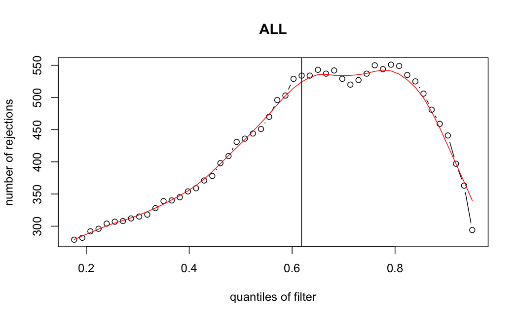
I honestly don't know what I'm really looking at here, but both these figures look wildly different with the example in the Bioconductor vignette.
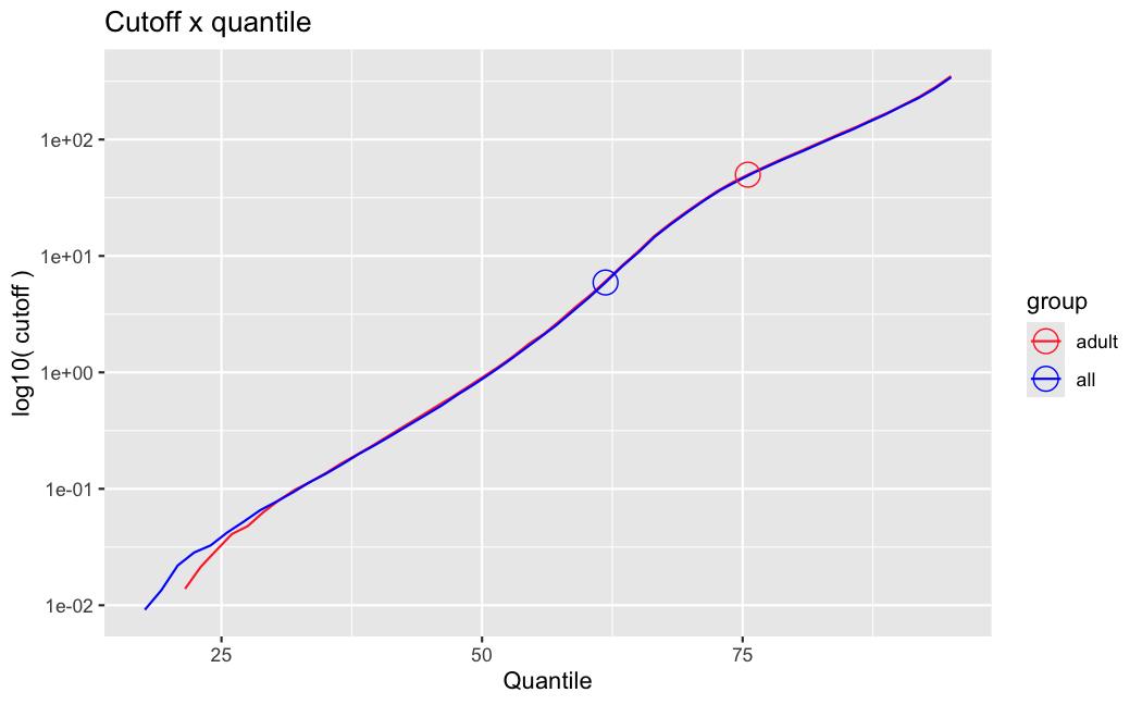
- Filter threshold
ADULT samples
> metadata(res_adult)$filterThreshold
75.5017%
49.8858

# "natural" pval = NAs
> summary(res_adult[is.na(res_adult$pvalue),]$baseMean)
     Min.   1st Qu.    Median      Mean   3rd Qu.      Max.
  0.00000   0.00000   0.00000   0.08045   0.00000 133.13102

# pval != NA, but padj = NA
> summary(res_adult[!is.na(res_adult$pvalue) & is.na(res_adult$padj),]$baseMean)
    Min.  1st Qu.   Median     Mean  3rd Qu.     Max.
 0.01763  0.13640  0.73736  6.59878  6.21863 49.88463

# padj != NA
> summary(res_adult[!is.na(res_adult$pvalue) & !is.na(res_adult$padj),]$baseMean)
    Min.  1st Qu.   Median     Mean  3rd Qu.     Max.
   49.89    87.80   153.62   350.21   296.26 44713.67
ALL samples
> metadata(res_all)$filterThreshold
61.8497%
5.917652

# "natural" pval = NAs
> summary(res_all[is.na(res_all$pvalue),]$baseMean)
    Min.  1st Qu.   Median     Mean  3rd Qu.     Max.
 0.00000  0.00000  0.00000  0.06754  0.00000 74.84557

# pval != NA, but padj = NA
> summary(res_all[!is.na(res_all$pvalue) & is.na(res_all$padj),]$baseMean)
   Min. 1st Qu.  Median    Mean 3rd Qu.    Max.
0.01110 0.06538 0.23794 0.82457 0.97549 5.91727

# padj != NA
> summary(res_all[!is.na(res_all$pvalue) & !is.na(res_all$padj),]$baseMean)
    Min.  1st Qu.   Median     Mean  3rd Qu.     Max.
    5.92    30.31    80.68   231.81   196.71 42934.59
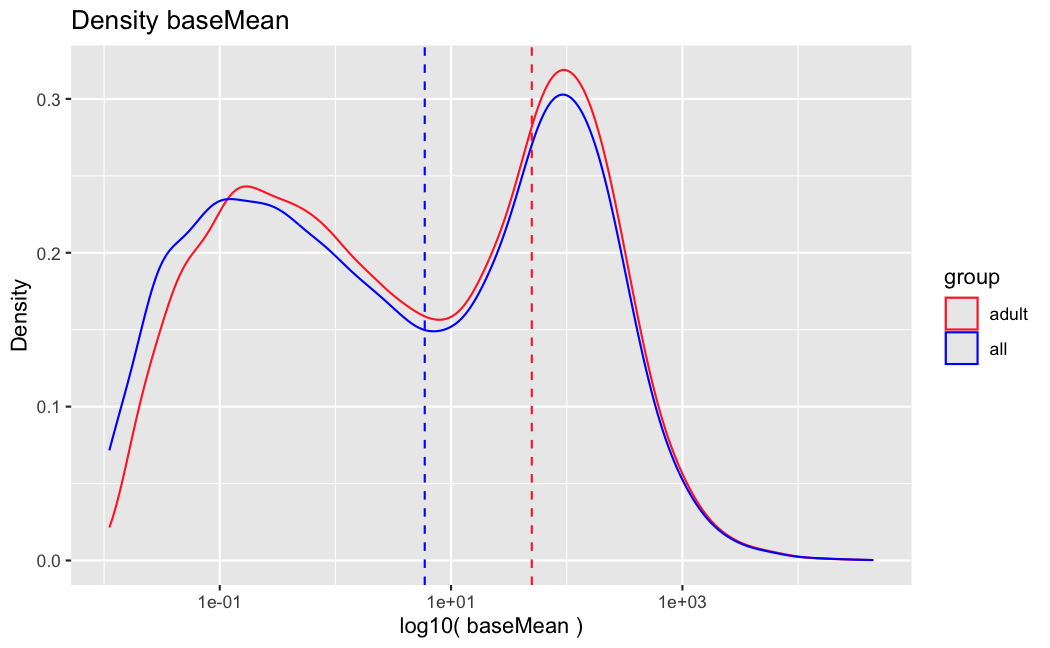
I don't know what I should be expecting here, but having the baseMean threshold jump from 5.9 to 49.8 looks like the exact reason why these genes are being excluded from the analysis.
It seems it is clearly driven by the independent filtering.
use <- res_all$baseMean > metadata(res_all)$filterThreshold
h1 <- hist(res_all$pvalue[!use], breaks=0:50/50, plot=FALSE)
h2 <- hist(res_all$pvalue[use], breaks=0:50/50, plot=FALSE)
colori <- c(`do not pass`="khaki", `pass`="powderblue")
barplot(height = rbind(h1$counts, h2$counts), beside = FALSE,
        col = colori, space = 0, main = "ALL", ylab="frequency")
text(x = c(0, length(h1$counts)), y = 0, label = paste(c(0,1)),
     adj = c(0.5,1.7), xpd=NA)
legend("topleft", fill=rev(colori), legend=rev(names(colori)))
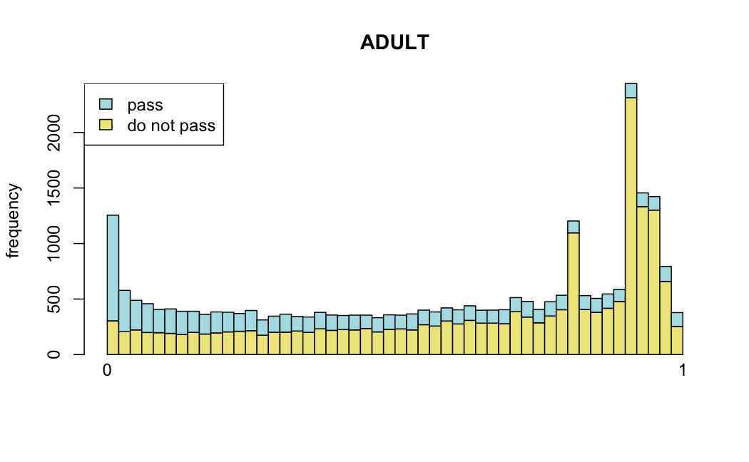
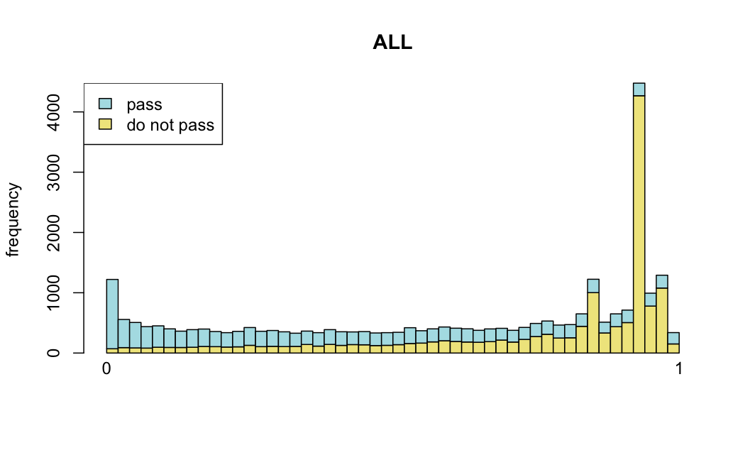
Which are, again, wildly different from what is described in the vignette
It seems clear that the choice of sample subsetting (or not) causes a change in the baseMean of the gene, but, most importantly, in the minimum baseMean threshold that the independent filter uses to remove genes from the analysis.
What am I really looking at here? What numbers should I be expecting here? Is a baseMean filter of 49.8 reasonable or is it extremely high? Should I keep using for the analysis only the ADULT samples, or should I convince my coauthors to use ALL the samples? (that might bias other interesting genes, though, I think that's in fact why we ended up choosing the ADULT subset).
Or is there something weird in this data that caused the independentFiltering to go crazy and I should simply ignore it and re-run the analysis with results(dds, independentFiltering=FALSE) ? Should I just leave it be and mention that these two genes are significantly up/down-regulated but their dispersion is too high to give an accurate log2FC estimate?
Thanks in advance

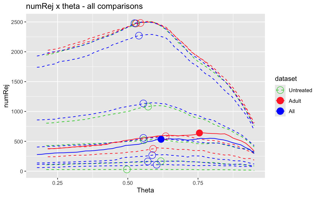
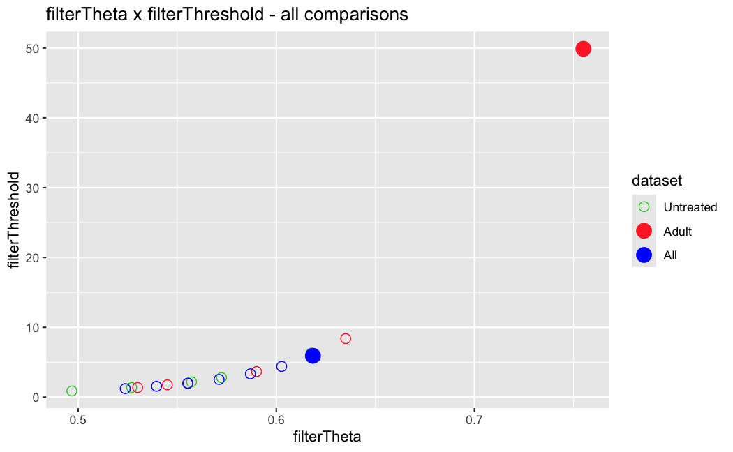
I have been back to this after a break. I have run a series of pairwise comparisons using either all the samples together, or only a subset-of-interest of them. Then I looked at how
filterThresholdchanged on each of them:(
modelvaris how I named the grouping variable, and I used adesign = modelvar+sexbecause there is a (balanced) mix of male and female mice)(The Untreated group only includes AL (control) samples both young and adult; the Adult group only includes Adult (22wk) samples both control and treated)
As you can see, only the
modelvar_22DminDR_vs_22DminALshows a relevant change infilterThreshold, but the new threshold is set to levels that I would deem unacceptably high. The rest of comparisons show very stable (and low) threshold levels.Sex also shows an increase in that threshold, but it is 5x smaller, and it makes sense because sex-associated genes are more highly expressed in adults than in younger mice.
I have worked around this by applying the threshold I got when using All samples to the results of the same comparison in the Adult subset, and then calculating the adjusted p-value for the genes passing the new (lower) threshold:
This gives me:
Out of 378 significant genes (
padj), 57 were significant with the old (high) threshold, but are no longer significant after multiple correction. They all had weak adjusted p-values very close to 0.05, that now are slightly above that.Out of 372 significant genes (
new_padj), 51 were previously deemedpadj = <NA>, and are now significant, with 15 genes with new_padj < 0.01.Is this the correct way to go about it?
And, most importantly, how can I prevent this from happening again? I am afraid that some of the analyses I did in the past might be facing this issue? Should I be paranoid and store the
filterThresholdof each comparison I run in DESeq2 moving forward and check them in case I find another super-high threshold like this one?Just saw this post, for some reason I didn't get it the first time.