
Hello,
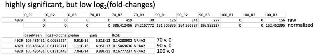
I am running DESeq2 from bulk RNA sequencing data. Our lab has a legacy pipeline for identifying differentially expressed genes, but I have recently updated it to include functionality such as lfcshrink(). I noticed that in the past, graduate students would use a pre-filter to eliminate genes that were likely not biologically meaningful, as many samples contained drop-outs and had lower counts overall. An example is attached here in my data, specifically, where this gene was considered significant:
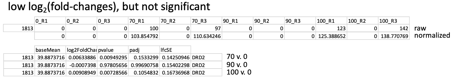
I also see examples of the other end of the spectrum, where I have quite a few dropouts, but this time there is no significant difference detected, as you can see here:
I have read in the vignette and the forums how pre-filtering is not necessary (only used to speed up the process), and that independent filtering should take care of these types of genes. However, upon shrinking my log2(fold-changes), I have these strange lines that appear on my volcano plots. I am attaching these, here:
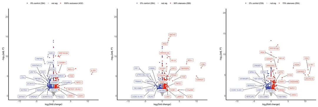
I know that DESeq2 calculates the log2(fold-changes) before shrinking, which is why this may appear a little strange (referring to the string of significant genes in a straight line at the volcano center). However, my question lies in why these genes are not filtered out in the first place? I can do it with some pre-filtering (I have seen these genes removed by adding a rule that 50/75% of samples must have a count greater than 10), but that seems entirely arbitrary and unscientific. All of these genes have drop-outs and low counts in some samples. Can you adjust the independent filtering, then? Is that the better approach? Or would applying an lfcthreshold() be better? Mind you, I am performing gene set enrichment analysis directly after this (with normalized counts directly from DESeq2), if that changes anything. I am continuously reading the vignette to try to uncover this answer. Still, as someone in the field with limited experience, I want to ensure I am doing what is scientifically correct.
I have attached relevant pieces of my code that may be useful. I snipped out any portions for visualizations, etc. to make it cleaner:
# Create coldata
coldata <- data.frame(
  row.names = sample_names,
  occlusion = factor(occlusion, levels = c("0", "70", "90", "100")),
  region = factor(region, levels = c("upstream", "downstream")),
  replicate = factor(replicate)
)

# Create DESeq2 dataset
dds <- DESeqDataSetFromMatrix(
  countData = cts,
  colData = coldata,
  design = ~ region + occlusion

# Filter genes with low expression ()
keep <- rowSums(counts(dds) >=10) >=12 # Have been adjusting this to view volcano plots differently
dds <- dds[keep, ]

# Run DESeq normalization
dds <- DESeq(dds)

# Load apelgm for LFC shrinkage
if (!requireNamespace("apeglm", quietly = TRUE)) {
  BiocManager::install("apeglm")
}
library(apeglm)

# 0% vs 70%
res_70 <- lfcShrink(dds, coef = "occlusion_70_vs_0", type = "apeglm")
write.table(
  cbind(res_70[, c("baseMean", "log2FoldChange", "pvalue", "padj", "lfcSE")],
        SYMBOL = mcols(dds)$SYMBOL),
  file = "06042025_res_0_vs_70.txt", sep = "\t", row.names = TRUE, col.names = TRUE
)

# 0% vs 90%
res_90 <- lfcShrink(dds, coef = "occlusion_90_vs_0", type = "apeglm")
write.table(
  cbind(res_90[, c("baseMean", "log2FoldChange", "pvalue", "padj", "lfcSE")],
        SYMBOL = mcols(dds)$SYMBOL),
  file = "06042025_res_0_vs_90.txt", sep = "\t", row.names = TRUE, col.names = TRUE
)

# 0% vs 100%
res_100 <- lfcShrink(dds, coef = "occlusion_100_vs_0", type = "apeglm")
write.table(
  cbind(res_100[, c("baseMean", "log2FoldChange", "pvalue", "padj", "lfcSE")],
        SYMBOL = mcols(dds)$SYMBOL),
  file = "06042025_res_0_vs_100.txt", sep = "\t", row.names = TRUE, col.names = TRUE
)
Thanks for your assistance! I hope I included everything necessary and am not repeating information found elsewhere on this forum. I scanned a lot, but couldn't find the exact keywords to find it (if it's out there).
EDIT: 06/10/2025 to include lfcthreshold() as an option in my title/body text

Dr. Love,
Thank you for the support. Is there a hard-and-fast rule for choosing a threshold in bulk RNAseq analyses using lfcthreshold()? As I understand it, most people will apply what works best for their data (after consulting threads such as: Effect of lfcThreshold on p-value in DESeq2).
Take care.
It has to come from the biology. What is a meaningful fold change in the system. Depending on context that could be doubling (1) or increasing by 50% (
log2(1.5)).Hi Dr. Love,
I believe I found some old forums that you had referenced earlier and used their suggestions, plus the advice given in this post, to try to get things to look correct. I ran some testing on a single comparison of mine (looking at just my control vs. 90% stenosis for now). I ended up using your first (of two) suggestions found on this forum post and am still encountering similar issues. Here is the code structure for the first suggestion:
As you can see in my attached volcano plot, after performing a threshold prior to a shrinkage, I still have a clump of genes that form that solid line in the very center of the plot:
Moreover, if I follow the second suggestion from that post (again, just using my 0% vs. 90% comparison for simplicity at the moment), my code structure turns into this:
I can then plot my s-values on my volcano plot instead of the adjusted p-values. I also compared how the s-values related to the adjusted p-values. For the volcano plot, I arbitrarily chose s = 0.05 for the time being to deem "significance." I have attached those images here: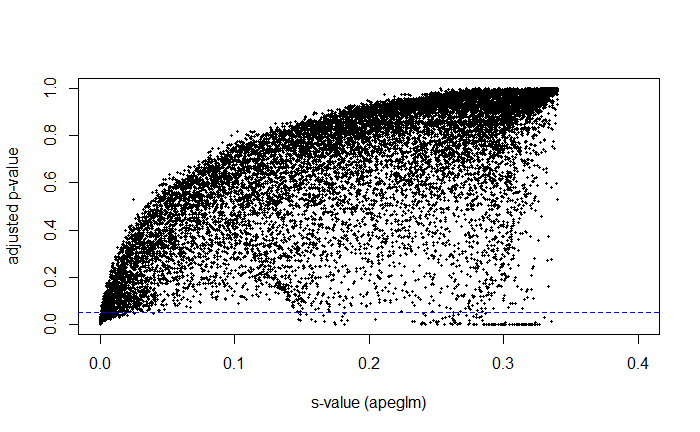
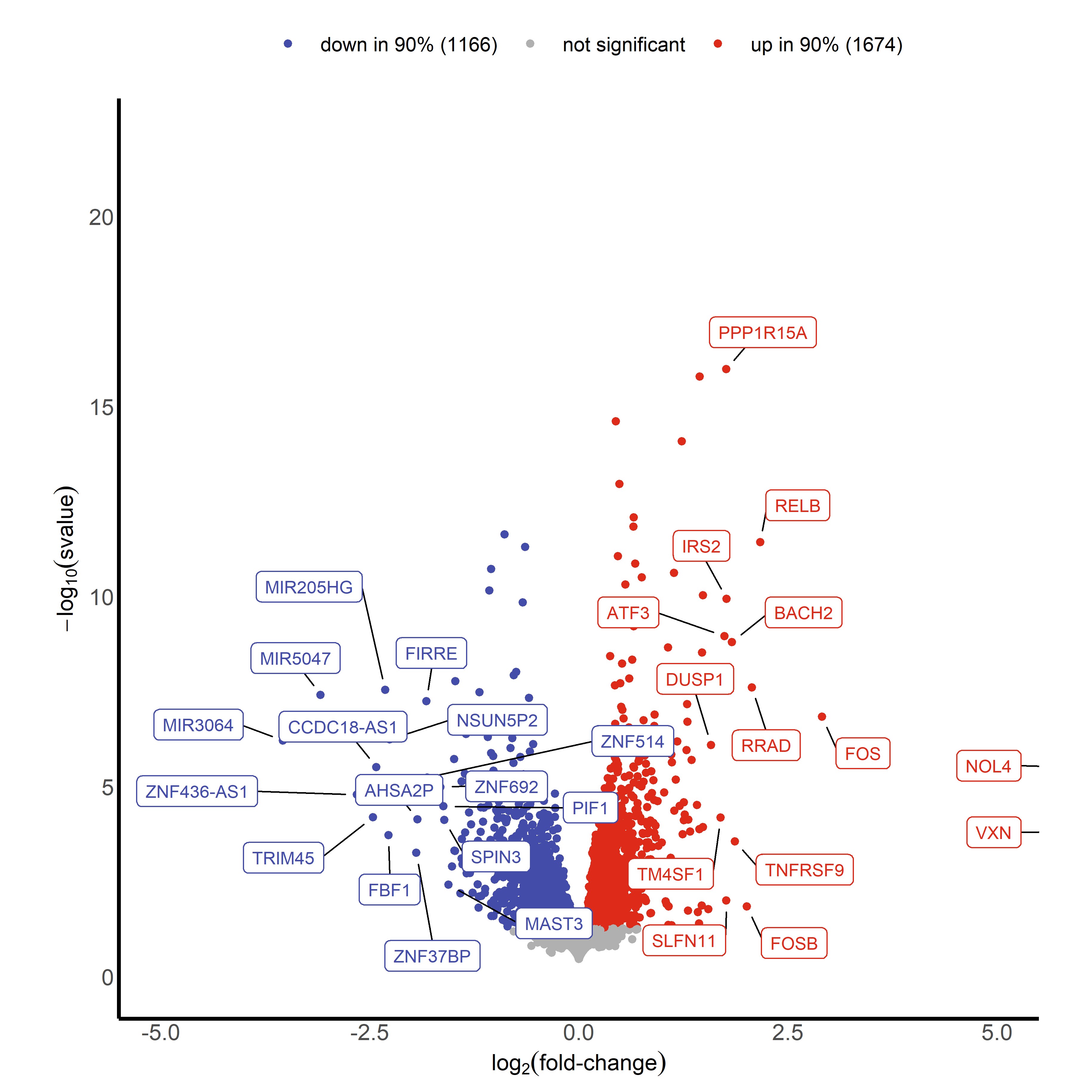
Finally, I can also add the thresholding argument that is built into lfcshrink(). I chose a biologically meaningful fold change of 50%, so I made the threshold to be 0.5850 and plotted the volcano plot (shown below). This dramatically reduced the number of "significant" genes, and might have been too stringent.
I understand that the s-value provides a measure of the false sign rate, which is the estimated probability that the sign of the log fold change estimate is wrong. What I want to ensure is how this can be used (and cutoff at suggested values of 0.01 or 0.005) instead of an adjusted p-value, which is traditionally used to determine significance. I read in Stephen's 2016 paper that having high confidence in a sign's correctness implies we also have high confidence in the number not being 0, which is considered "signless." Is that a correct interpretation?
This is a direct quote from the paper that gave me that interpretation:
I do not have a statistics background whatsoever, but I believe my interpretation is correct? After graphing, it is evident that s-values and adjusted p-values correlate relatively well. With a strict cut-off, all s-values below a particular threshold would almost 100% be below 0.05 in their adjusted p-value.
The big question: Would simply reporting s-values in the volcano plots be the best approach in the future (and even disregard thresholding)? And would adding a threshold of s-values to highlight genes of interest in heat maps be appropriate? My intuition is yes, mainly because the approach tends to be more conservative than traditional adjusted p-values, and is readily accepted in your field. But then this raises the question... why would we not just use s-values over adjusted p-values all the time? Is there still debate about prioritizing type S errors over type I errors in these statistical analyses?
Thank you so much as always!
EDIT: 06/24/2025 to rephrase some of my paragraphs after doing some additional reading
There is no problem with reporting the s-values with the volcano plots from lfcShrink. No reason not to use these, and with the increasing use of ashr I think they are more widely known now.