In the analysis of the gene expression in a model with two genotypes and infection factor, I've got into a strange behaviour of the model fitting. In the full scenario this happened for couple of genes out of the full genome. Here I stripped the data to 4 genes -- 3 "good" ones, and on "bad".

The experiment has expression data of two genotypes with infection A (no infection) and infection B. The goal is to see if there is difference in reaction to infection B between the two genotypes.

library(DESeq2)

## Data -- real world example, stripped down to 4 genes
count_matrix <- matrix(c(0L, 340L, 79L, 817L,
                         0L, 294L, 43L, 244L,
                         0L, 439L, 39L, 501L,
                         11L, 648L, 26L, 506L,
                         2L, 274L, 25L, 196L,
                         3L, 432L, 20L, 471L,
                         4L, 186L, 28L, 452L,
                         242L, 292L, 16L, 287L,
                         3L, 9L, 0L, 31L,
                         0L, 86L, 19L, 268L,
                         5L, 626L, 29L, 440L,
                         0L, 183L, 10L, 290L,
                         10L, 172L, 53L, 570L,
                         1L, 256L, 20L, 216L,
                         137L, 90L, 13L, 118L,
                         0L, 110L, 1L, 56L,
                         0L, 11L, 1L, 36L,
                         3L, 583L, 43L, 453L,
                         4L, 177L, 12L, 326L,
                         0L, 480L, 30L, 739L),
                       nrow = 4,
                       dimnames = list(c("g1", "g2", "g3", "g4"), NULL))
## The samples are classified in two two-level factors.
cdat <- data.frame(genotype = structure(c(1L, 1L, 1L, 1L, 1L, 1L, 2L, 2L, 2L, 2L, 2L, 2L, 2L, 2L, 2L, 2L, 2L, 2L, 2L, 2L),
                                        levels = c("NT", "TR"), class = "factor"),
                   infection = structure(c(1L, 1L, 1L, 2L, 2L, 2L, 1L, 1L, 1L, 1L, 1L, 1L, 1L, 2L, 2L, 2L, 2L, 2L, 2L, 2L),
                                         levels = c("A", "B"), class = "factor"))
## Combine all factor combinations into individual groups
cdat$group <- factor(paste0(cdat$genotype, ".", cdat$infection))

To get the interesting effect, I tried two approaches -- the suggested in the tutorial "simple" way of fitting the model where group is all possible combinations of the factors, and then manually constructing the interesting contrast.

I also made a "complicated" formula with factor interaction. I would expect the results to coincide up to numerical rounding errors.

de <- DESeqDataSetFromMatrix(count_matrix, cdat, design = ~group)
de <- DESeq(de)

de2 <- DESeqDataSetFromMatrix(count_matrix, cdat, design = ~genotype*infection)
de2 <- DESeq(de2)

In the "by group" approach, the difference in infection response in genotypes TR and NT is given by a contrast (TR.B-TR.A) - (NT.B-NT.A) (Note, that the NT.A is actually intercept, so nothing to be subtracted in the first value)

resultsNames(de)
res <- results(de, contrast=c(0, -1, -1, 1))
res[order(res$pvalue),]

## log2 fold change (MLE): 0,-1,-1,+1 
## Wald test p-value: 0,-1,-1,+1 
## DataFrame with 4 rows and 6 columns
##     baseMean log2FoldChange     lfcSE       stat      pvalue        padj
##    <numeric>      <numeric> <numeric>  <numeric>   <numeric>   <numeric>
## g1   27.3903    -16.6982964  3.576776 -4.6685332 3.03358e-06 1.21343e-05
## g3   17.7412      0.6863586  0.697873  0.9835013 3.25361e-01 6.50722e-01
## g2  198.4733      0.0149538  0.383796  0.0389630 9.68920e-01 9.73736e-01
## g4  272.1577      0.0125052  0.379825  0.0329235 9.73736e-01 9.73736e-01

As a result "g1" is quite significant, with large log2FC.

Let us repeat the analysis in "factor interaction approach", where the result is just one of the formula coefficients

resultsNames(de)
res2 <- results(de2, name="genotypeTR.infectionB")
res2[order(res2$pvalue),]
## log2 fold change (MLE): genotypeTR.infectionB 
## Wald test p-value: genotypeTR.infectionB 
## DataFrame with 4 rows and 6 columns
##     baseMean log2FoldChange     lfcSE       stat    pvalue      padj
##    <numeric>      <numeric> <numeric>  <numeric> <numeric> <numeric>
## g1   27.3903     -4.3205263  3.576733 -1.2079532  0.227065  0.650721
## g3   17.7412      0.6863583  0.697872  0.9835014  0.325361  0.650721
## g2  198.4733      0.0149538  0.383796  0.0389630  0.968920  0.973736
## g4  272.1577      0.0125052  0.379825  0.0329235  0.973736  0.973736

The difference for "g1" is much smaller!

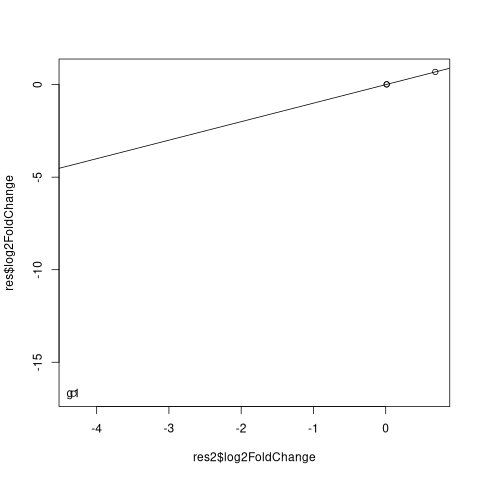
Note, to check that I am not mistaking with contrasts, we can see that for other genes the log2FC is the same in both approaches

plot(res2$log2FoldChange, res$log2FoldChange)
abline(a=0,b=1)
res_ne <- abs(res$log2FoldChange-res2$log2FoldChange)>0.01
text(res2$log2FoldChange[res_ne], res$log2FoldChange[res_ne], rownames(res)[res_ne])

To analyse the source of difference in the fits, one can see, that the fits of mu are different for g1 in the NT.A category, where the count signal is zero.

Here I plot (normalized) counts for g1 together with (normalized) mu values

op <- par(mfrow=c(1,2))
plotCounts(de, gene=1, intgroup="group", pc=0.5, main="By group fits for g1")
points(colData(de)$group, assay(de, "mu")[1,]/sizeFactors(de)+0.5, type="h")
##
plotCounts(de2, gene=1, intgroup="group", pc=0.5, main="factor interaction fits for g1")
points(colData(de2)$group, assay(de2, "mu")[1,]/sizeFactors(de2)+0.5, type="h")
par(op)

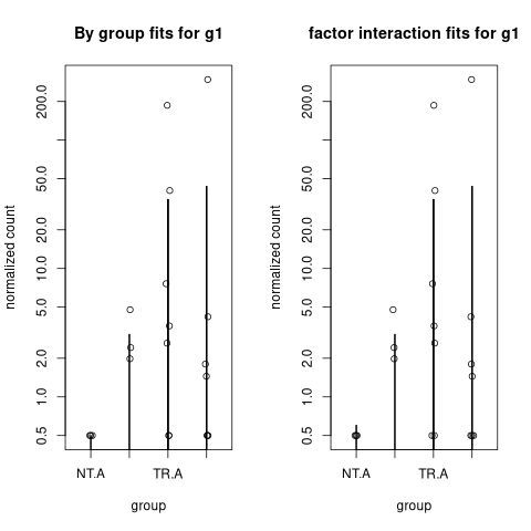
What we can see, that in the case of individual groups the for created small value of mu for NT.A group, while the factor interaction was constrained giving normalized mu fit around 0.1

assay(de, "mu")[1,]/sizeFactors(de)
## [1] 1.901766e-05 1.901766e-05 1.901766e-05 2.569091e+00 2.569091e+00 2.569091e+00 3.400778e+01 3.400778e+01 3.400778e+01 3.400778e+01 3.400778e+01 3.400778e+01 3.400778e+01 4.320288e+01 4.320288e+01 4.320288e+01 4.320288e+01
33 [18] 4.320288e+01 4.320288e+01 4.320288e+01

assay(de2, "mu")[1,]/sizeFactors(de2)
## [1]  0.1012012  0.1012012  0.1012012  2.5691565  2.5691565  2.5691565 34.0054435 34.0054435 34.0054435 34.0054435 34.0054435 34.0054435 34.0054435 ## 43.2061381 43.2061381 43.2061381 43.2061381 43.2061381 43.2061381 43.2061381

Actually, further study shows, that there is minmu parameter for DESeq, and setting it to the small value allows to reproduce the "by group" result from "factor interaction" approach

de2_smallmu <- DESeq(de2, minmu=1e-6)
assay(de2_smallmu, "mu")[1,]/sizeFactors(de2_smallmu)

However, it does not work another way around -- fitting the "by group" model with large minmu does not change anything (this is expected, as far as 0.5 is the default value for minmu).

de_largemu <- DESeq(de, minmu=0.5)
assay(de_largemu, "mu")[1,]/sizeFactors(de_largemu)

In my understanding, the fit in the "by group" formula does something wrong in this case. Note, that this result is stable over several versions of R/Bioconductor.

Note also, that adding 0 to prevent intercept in formulas does not change the fits.

Any ideas what causes this behaviour? The results obtained in "factor interaction" approach are the ones that seem biologically relevant for me, while "by group" approach gives "g1" as an artefact. For the current project I am continuing with "factor interaction", but it is a bit uncomfortable to know that sometimes genes with zerop expression in one condition give rise to artefacts.

sessionInfo( )

This has been noted before on the support site, that when you compare two groups with 0 counts, depending on the design, the coefficients are different.

If you use contrast with named groups to compare, results() will zero out the LFC when you compare two groups with all zero counts, but this behavior isn't applied when you use a different but equivalent design.

My recommendation usually is to see if you really want to include such genes (not expressed in multiple groups). Likely it would make more sense to filter these as you will end up having to compare a finite LFC to an infinite LFC.