log2foldchange vs density plot from likelihood and posterior
1
0
Entering edit mode
@nnaharfancy-20022
Last seen 3.5 years ago
Imperial College London

Hi

I am trying to visualise the spread of the mean count from MLE calculation following DEseq2, 2014 paper and the attached codes from DEseq2paper package. The difference in my case is, instead of two different genes, I am plotting the likelihood data of the same gene from two dataset. The experiment design is as follows, I have three reps of control and three reps of treatment samples. From the same samples two types of library was prepared mRNA (NEB for illumina) and lexogen quantseq (3 prime end). The idea is to compare the efficiency of two library preparation method to detect DGEs. The quantseq yielded 60% of the DGEs detected by NEB mRNA. Now I am exploring more to check the propertied of the genes that are not called DGEs by quantseq.So, many of them were low counts. That is one reason, another reason could be high dispersion. To visualise the disperson and compare the MLE from both method I am plotting gene by gene.

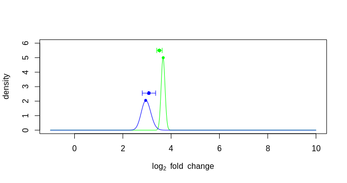
The issue I am having is the lfc from the result table and the mle from plot has difference more than 0.01 and there I am getting an error. Please see the code below. So, I am plotting the error bar position using the beta beta value corresponding to maximum MLE value. But why they are so much offset?

Thanks for any help.

betas <- seq(from=-1,to=10,length=500)
cond <- as.numeric(colData(dds.standard)$Treatment) - 1

likelihood <- function(k,alpha,intercept) {
  z <- sapply(betas,function(b) {
    prod(dnbinom(k,mu=sf*2^(intercept + b*cond),size=1/alpha))
  })
  z/sum(z * diff(betas[1:2]))
}

points2 <- function(x,y,col="black",lty) {
  points(x,y,col=col,lty=lty,type="l")
  points(x[which.max(y)],max(y),col=col,pch=20)
}

lfc1 <- res.standard["ICAM1",]$log2FoldChange
lfc2 <- res.three["ICAM1",]$log2FoldChange
lfc <- c(lfc1, lfc2)

k1 = counts(dds.standard)["ICAM1", ]
k2 = counts(dds.three)["ICAM1", ]
cond <- as.numeric(colData(dds)$Treatment) - 1
a1 = dispersions(dds.standard["ICAM1",])
a2 = dispersions(dds.three["ICAM1", ])
ints1 <- mcols(dds.standard["ICAM1",])$Intercept
ints2 <- mcols(dds.three["ICAM1",])$Intercept

lfcSE1 <- results(dds.standard["ICAM1",])$lfcSE
lfcSE2 <- results(dds.three["ICAM1",])$lfcSE
lfcSE <- c(lfcSE1, lfcSE2)

sf = sizeFactors(dds.standard)
density1 <- likelihood(k1,a1,ints1)
sf = sizeFactors(dds.three)
density2 <- likelihood(k2,a2,ints2)

position1 <- betas[which.max(density1)]
position2 <- betas[which.max(density2)]
position <- c(position1, position2)

hghts1 <- max(density1)+0.5
hghts2 <- max(density2)+0.5
hghts <- c(hghts1, hghts2)

mleFromPlot <- c(position1, position2)
stopifnot(all(abs(lfc - mleFromPlot) < .01)) #Error: all(abs(lfc - mleFromPlot) < 0.01) is not TRUE

plot(betas,likelihood(k1,.5,4),type="n",ylim=c(0,6),
     xlab=expression(log[2]~fold~change),
     ylab="density")
points2(betas,density1,lty=1,col="green")
points2(betas,density2,lty=1,col="blue")
points(position, hghts, col=c("green", "blue"), pch=16)
arrows(position, hghts, position + lfcSE, hghts, col=c("green", "blue"), length=.05, angle=90)
arrows(position, hghts, position - lfcSE, hghts, col=c("green", "blue"), length=.05, angle=90)
mtext(side=3,line=line,adj=adj,cex=cex)

> sessionInfo()
R version 3.6.1 (2019-07-05)
Platform: x86_64-pc-linux-gnu (64-bit)
Running under: Ubuntu 18.04.2 LTS

Matrix products: default
BLAS:   /usr/lib/x86_64-linux-gnu/blas/libblas.so.3.7.1
LAPACK: /usr/lib/x86_64-linux-gnu/lapack/liblapack.so.3.7.1

locale:
 [1] LC_CTYPE=en_GB.UTF-8       LC_NUMERIC=C               LC_TIME=en_GB.UTF-8       
 [4] LC_COLLATE=en_GB.UTF-8     LC_MONETARY=en_GB.UTF-8    LC_MESSAGES=en_GB.UTF-8   
 [7] LC_PAPER=en_GB.UTF-8       LC_NAME=C                  LC_ADDRESS=C              
[10] LC_TELEPHONE=C             LC_MEASUREMENT=en_GB.UTF-8 LC_IDENTIFICATION=C       

attached base packages:
[1] parallel  stats4    stats     graphics  grDevices utils     datasets  methods   base     

other attached packages:
 [1] ggplot2_3.1.1               DESeq2_1.24.0               SummarizedExperiment_1.14.0
 [4] DelayedArray_0.10.0         BiocParallel_1.18.0         matrixStats_0.54.0         
 [7] Biobase_2.44.0              GenomicRanges_1.36.0        GenomeInfoDb_1.20.0        
[10] IRanges_2.18.0              S4Vectors_0.22.0            BiocGenerics_0.30.0        

loaded via a namespace (and not attached):
 [1] bit64_0.9-7            splines_3.6.1          Formula_1.2-3          assertthat_0.2.1      
 [5] latticeExtra_0.6-28    blob_1.1.1             GenomeInfoDbData_1.2.1 pillar_1.4.0          
 [9] RSQLite_2.1.1          backports_1.1.4        lattice_0.20-38        glue_1.3.1            
[13] digest_0.6.18          RColorBrewer_1.1-2     XVector_0.24.0         checkmate_1.9.3       
[17] colorspace_1.4-1       htmltools_0.3.6        Matrix_1.2-17          plyr_1.8.4            
[21] XML_3.98-1.19          pkgconfig_2.0.2        genefilter_1.66.0      zlibbioc_1.30.0       
[25] purrr_0.3.2            xtable_1.8-4           scales_1.0.0           htmlTable_1.13.1      
[29] tibble_2.1.1           annotate_1.62.0        withr_2.1.2            nnet_7.3-12           
[33] lazyeval_0.2.2         survival_2.44-1.1      magrittr_1.5           crayon_1.3.4          
[37] memoise_1.1.0          foreign_0.8-71         tools_3.6.1            data.table_1.12.2     
[41] stringr_1.4.0          munsell_0.5.0          locfit_1.5-9.1         cluster_2.1.0         
[45] AnnotationDbi_1.46.0   compiler_3.6.1         rlang_0.3.4            grid_3.6.1            
[49] RCurl_1.95-4.12        rstudioapi_0.10        htmlwidgets_1.3        bitops_1.0-6          
[53] base64enc_0.1-3        gtable_0.3.0           DBI_1.0.0              R6_2.4.0              
[57] gridExtra_2.3          knitr_1.22             dplyr_0.8.0.1          bit_1.1-14            
[61] Hmisc_4.2-0            stringi_1.4.3          Rcpp_1.0.1             geneplotter_1.62.0    
[65] rpart_4.1-15           acepack_1.4.1          tidyselect_0.2.5       xfun_0.6   

  1. plotting error bar using betas

  2. plotting error bar using lfc

deseq2 • 1.3k views
ADD COMMENT
0
Entering edit mode

plot using betas for standard error bar position

plot with lfc for error position

ADD REPLY
1
Entering edit mode
@mikelove
Last seen 13 hours ago
United States

This is quite a complex plot for a data analysis. In the paper it is used to give some intuition on how the Bayesian method for LFC works.

I'd recommend just plotting log2FoldChange +/- lfcSE, so as to make the plot easier to follow and easier to construct. And you should be using lfcShrink with type="apeglm" or "ashr", as these outperform the Normal prior as shown here:

https://academic.oup.com/bioinformatics/article/35/12/2084/5159452

ADD COMMENT
0
Entering edit mode

Hi Michael,

Thank you very much for commenting. I was secretly hoping that you will see my post.

So, you recommend to plot bar chart with lfcSE! And, do you think this is the right comparison I am doing as to find out why these genes are not called DGEs? For example I found among 715 DGEs that were not called as DGEs 31% (222) genes were very low count (basemean less then 10). For the rest I am thinking may be it is the dispersion. How can I actually prove that? Looking forward to hearing from you.

As you mentioned lfcshrink, I was also gonna ask, (I know in numerous post you mentioned it is for visualisation and ranking of the gene but I am asking again), which lfc should I report during publication shrunken or unsrhunken?

ADD REPLY
0
Entering edit mode

To figure out why a gene is not called DE, I typically look at plotCounts for various genes.

You can report either, but the shrunken LFC are better for ranking across all genes, at least in our benchmarks.

ADD REPLY
0
Entering edit mode

Say, for this particular case of STAT3, this is a very common gene to be found upregulated under LPS treatment (ou experiment from standard sequencing and previous literature) but failed to be DE in three-prime dataset. The count for this this is not particularly low nor the fold change is very different from the standard one. I am banging my head to find out an answer so that I can explain this or suggest some changes either in the analysis or in the library preparation step ( for example, increasing RNA quantity as a starting material). I know these two are fundamentally different library preparation but missing 40% DE seems to be quite a lot.

The lfcSE is almost double here, and the dispersion values are as follows

I will really appreciate any suggestion or direction.

dds.standard <- DESeqDataSetFromMatrix(countData = Standard,
                              colData = SampleData.standard,
                              design = ~Subject+Treatment)
dds.standard <- estimateSizeFactors(dds.standard)
dds.standard <- DESeq(dds.standard)
res.standard <- results(dds.standard, lfcThreshold = 2, alpha = 0.05)
res.standard.shrunk <- lfcShrink(dds.standard,  coef = 4, lfcThreshold = 2, type = "apeglm", svalue = FALSE )
> dispersions(dds.standard["STAT3", ])
[1] 0.01399543
res.standard["STAT3", ]
log2 fold change (MLE): Treatment LPS vs Control 
Wald test p-value: Treatment LPS vs Control 
DataFrame with 1 row and 6 columns
              baseMean  log2FoldChange            lfcSE             stat               pvalue
             <numeric>       <numeric>        <numeric>        <numeric>            <numeric>
STAT3 16372.9732823044 2.4750855697845 0.13994242659361 3.39486445496715 0.000686625849295624
                    padj
               <numeric>
STAT3 0.0077643232565498


dds.three <- DESeqDataSetFromMatrix(countData = Three.prime,
                              colData = SampleData.three.prime,
                              design = ~Subject+Treatment)
dds.three <- estimateSizeFactors(dds.three)
dds.three <- DESeq(dds.three)
res.three <- results(dds.three, lfcThreshold = 2, alpha = 0.05)
res.three.shrunk <- lfcShrink(dds.three, coef = 4, lfcThreshold = 2, type = "apeglm", svalue = FALSE)
> dispersions(dds.three["STAT3", ])
[1] 0.04221533
> res.three["STAT3", ]
log2 fold change (MLE): Treatment LPS vs Control 
Wald test p-value: Treatment LPS vs Control 
DataFrame with 1 row and 6 columns
              baseMean   log2FoldChange             lfcSE             stat            pvalue
             <numeric>        <numeric>         <numeric>        <numeric>         <numeric>
STAT3 4443.04649165151 2.34662946416062 0.243241498387395 1.42504246380101 0.154144926678722
           padj
      <numeric>
STAT3         1

  1. standard count
  2. three prime count

standard three.prime

ADD REPLY
0
Entering edit mode

You seem to be using a really large lfcThreshold. You’re setting less than four fold to be null. This particular gene is about four fold. I’d recommend using a much smaller LFC threshold.

ADD REPLY
0
Entering edit mode

Thank you Michael, you are right. But that will increase the number of DGEs proportionally for the standard dataset right? Which property of the dataset is driving this discrepency? How can I understand more about the dataset property?

ADD REPLY
0
Entering edit mode

Here I can answer software related questions but don’t have much extra time to help with interpretation of results per dataset. As far as the reason for the large pvalue, I think we’ve arrived at the answer.

ADD REPLY

Login before adding your answer.

Traffic: 550 users visited in the last hour
Help About
FAQ
Access RSS
API
Stats

Use of this site constitutes acceptance of our User Agreement and Privacy Policy.

Powered by the version 2.3.6