EDASeq normalization: genes with 0 counts
1
0
Entering edit mode
gprezza • 0
@611515a7
Last seen 13 days ago
Germany

I am analyzing an RNA-seq experiment in which I compare a control library (high coverage) with a treatment one (low coverage). There is some sample-specific length bias across samples and I am trying to correct this with the EDASeq package.

data <- newSeqExpressionSet(counts=as.matrix(reads[keep,]),
                            featureData=featureData,
                            phenoData=data.frame(
                                    conditions=conds,
                                    row.names=colnames(reads)))

dataOffset <- withinLaneNormalization(data,"length", which="full",offset=TRUE)
dataOffset <- betweenLaneNormalization(dataOffset, which="full",offset=TRUE)

After normalization, I do DGE analysis with edgeR:

a <- DGEList(counts=counts(dataOffset), group=conds, genes=as.character(rownames(reads[keep,])))
a$offset <- -offst(dataOffset)
a <- estimateDisp(a, design)
fit <- glmQLFit(a,design,robust=TRUE)

If we look at the volcano plot from the DGE analysis, there's a weird cluster of genes that are clearly separated from the "volcano": volcano plot

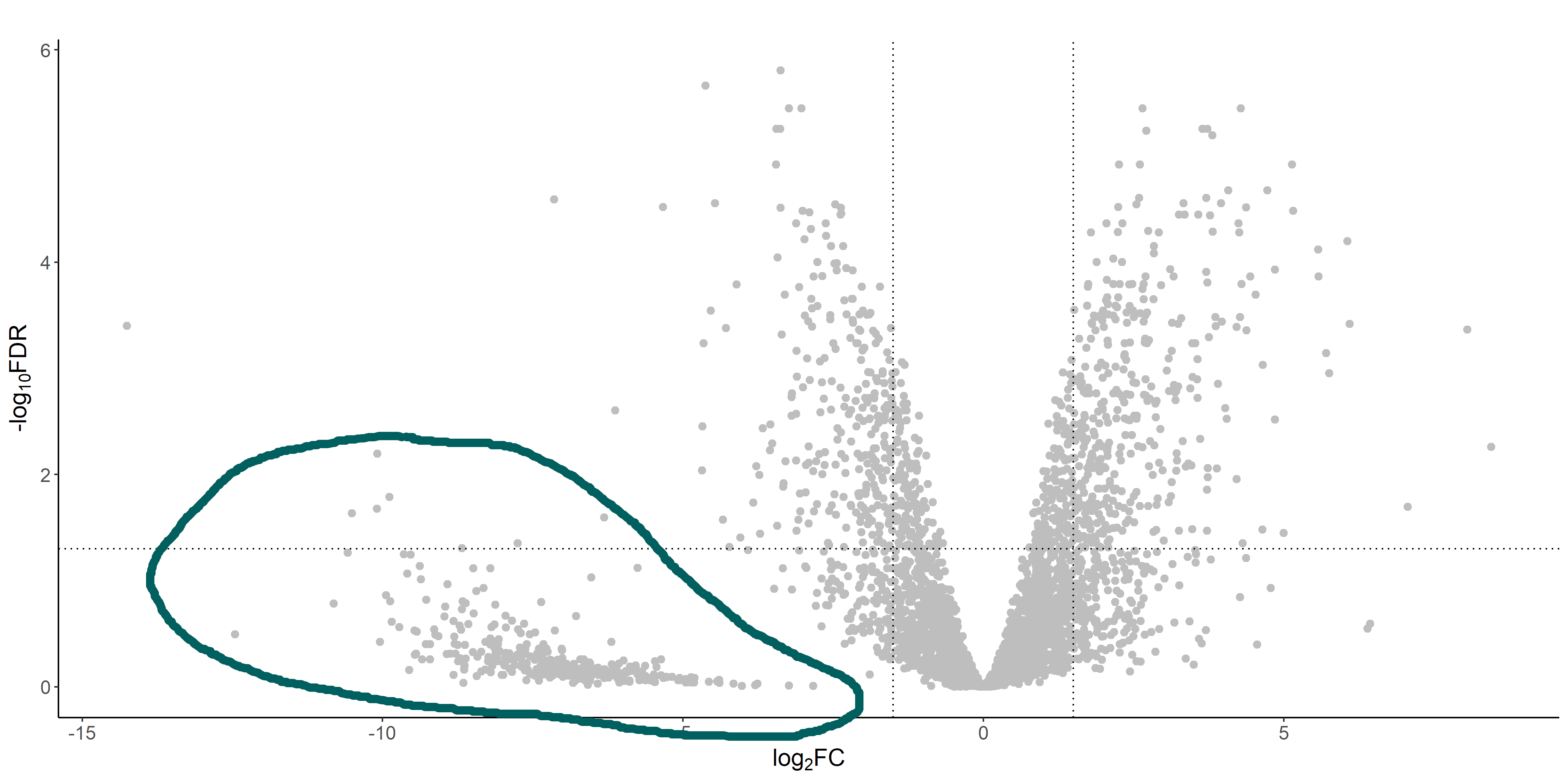
These genes are the ones that have 0 (or very low) read counts in the treatment library (which has a much lower coverage than the control one). If we look at the raw and normalized counts of these genes, I see that often they have originally 0 reads, but after normalization they get assigned with a discrete number of reads. This number is usually relatively different between replicates, and I guess that's why edgeR (correctly I guess) assigns a high FDR to these genes.

I am however a bit confused by how can a gene with 0 reads be assigned any number of reads after normalization. Is this something that is expected? I don't recall ever seeing a volcano plot with a separated cluster of genes as I am seeing now.

edgeR EDASeq • 1.2k views
ADD COMMENT
2
Entering edit mode
davide risso ▴ 950
@davide-risso-5075
Last seen 5 weeks ago
University of Padova

Hi,

you are using full-quantile normalization to normalize the data. This method matches the empirical distribution of all samples to that of a reference sample (usually taken as the median across all samples). If, as in your case, samples have very different coverages, it may happen that the zeroes are transformed in non-zero values.

As a (somewhat extreme) toy example, consider if you only had two samples and 6 genes that looked like this:

> x = matrix(c(0, 0, 1, 2, 4, 5, 10, 12, 12, 13, 14, 15), ncol=2)
> x
     [,1] [,2]
[1,]    0   10
[2,]    0   12
[3,]    1   12
[4,]    2   13
[5,]    4   14
[6,]    5   15

Because the median of 0 and 10 is 5, the first 0 will be transformed to 5 (and the second to 6).

> betweenLaneNormalization(x, which="full")
     [,1] [,2]
[1,]    5    5
[2,]    6    6
[3,]    6    6
[4,]    8    8
[5,]    9    9
[6,]   10   10

If you want to preserve the zeros in the normalized data, you have to use one of the many scaling normalizations available, for instance with upper-quartile scaling, the same toy example will look like this

> betweenLaneNormalization(x, which="upper")
     [,1] [,2]
[1,]    0    6
[2,]    0    8
[3,]    2    8
[4,]    5    8
[5,]   10    9
[6,]   12    9
attr(,"scaled:scale")
[1] 0.4057971 1.5942029

I hope this helps.

ADD COMMENT
0
Entering edit mode

This is very clear and it definitely helps. Thanks for taking the time to reply!

ADD REPLY

Login before adding your answer.

Traffic: 760 users visited in the last hour
Help About
FAQ
Access RSS
API
Stats

Use of this site constitutes acceptance of our User Agreement and Privacy Policy.

Powered by the version 2.3.6