
Problem with estimateSizeFactors due to avgTxLength
I believe there is a problem with estimateSizeFactors.DESeqDataSet, specifically where nm is created as the avgTxLength divided by the geometric means of avgTxLength:
    if ("avgTxLength" %in% assayNames(object)) {
      nm <- assays(object)[["avgTxLength"]]
      nm <- nm / exp(rowMeans(log(nm))) # divide out the geometric mean
      normalizationFactors(object) <- estimateNormFactors(counts(object),
                                                          normMatrix=nm,
                                                          locfunc=locfunc,
                                                          geoMeans=geoMeans,
                                                          controlGenes=controlGenes)
      if (!quiet) message("using 'avgTxLength' from assays(dds), correcting for library size")
avgTxLength per sample can vary quite dramatically according to isoform expression for that gene within each sample. Because the eventual normalizationFactors are scaled by this value via statement:
nf <- t( t(normMatrix) * sf )
where normMatrix is the nm from above, difference in isoform composition between samples can have a dramatic effect on the normalized reads.
I have a particular case that illustrates this issue. Gene ENSG00000069275.12 has two isoforms, one long and the other very short (e.g. Salmon Effective Length 6341 vs. 13). Depending on the expression of these two transcripts the resulting avgTxLength varies in my 16 samples between 160 and 1503. By dividing nm by the geometric mean of the avgTxLength (603 in this case), the resulting nm ranges between 0.27 and 2.49.
Since nm (normMatrix) carries all the way through to the final normalization factors:
nf <- t( t(normMatrix) * sf )
This results in large changes in Normalized counts. For example, in the sample with avgTxLength=160, the original counts were 17484 and the normalized counts were amplified to 75992, for the sample with the larger avgTxLength=1503 the original counts were 12739 and the normalized counts were reduced to 6013. Note that the library sizes are very similar, the changes are coming from nm due to different isoform distribution for this gene in the samples.
As a sanity check, I also processed the data again but this time zeroed out the counts and abundance for each of the two transcripts in turn. Here of course, avgTxLength is much more tightly bound (ranging from 5592 to 6396 for the longer transcript and 13 for the short one) and the resulting normalized read counts are close to the unnormalized values as expected.
This issue illustrated by this example is of course amplified by the difference in length between these two transcripts, but I question why the geometric means of the avgTxLength are used, as differences in isoform utilization between samples are affecting normalized reads in all cases.
Thank you,
Mark
sessionInfo( )

R version 4.0.3 (2020-10-10)
Platform: x86_64-pc-linux-gnu (64-bit)
Running under: Ubuntu 18.04.5 LTS

Matrix products: default
BLAS:   /usr/lib/x86_64-linux-gnu/blas/libblas.so.3.7.1
LAPACK: /usr/lib/x86_64-linux-gnu/lapack/liblapack.so.3.7.1

locale:
[1] C

attached base packages:
[1] parallel  stats4    stats     graphics  grDevices utils     datasets
[8] methods   base

other attached packages:
 [1] GenomicFeatures_1.42.3      AnnotationDbi_1.52.0
 [3] tximeta_1.8.4               DESeq2_1.30.1
 [5] SummarizedExperiment_1.20.0 Biobase_2.50.0
 [7] MatrixGenerics_1.2.1        matrixStats_0.58.0
 [9] GenomicRanges_1.42.0        GenomeInfoDb_1.26.4
[11] IRanges_2.24.1              S4Vectors_0.28.1
[13] BiocGenerics_0.36.0

loaded via a namespace (and not attached):
 [1] ProtGenerics_1.22.0           bitops_1.0-6
 [3] bit64_4.0.5                   RColorBrewer_1.1-2
 [5] progress_1.2.2                httr_1.4.2
 [7] repr_1.1.3                    tools_4.0.3
 [9] utf8_1.2.1                    R6_2.5.0
[11] lazyeval_0.2.2                DBI_1.1.1
[13] colorspace_2.0-0              withr_2.4.1
[15] tidyselect_1.1.0              prettyunits_1.1.1
[17] bit_4.0.4                     curl_4.3
[19] compiler_4.0.3                xml2_1.3.2
[21] DelayedArray_0.16.3           rtracklayer_1.50.0
[23] scales_1.1.1                  genefilter_1.72.1
[25] askpass_1.1                   rappdirs_0.3.3
[27] Rsamtools_2.6.0               pbdZMQ_0.3-5
[29] stringr_1.4.0                 digest_0.6.27
[31] XVector_0.30.0                base64enc_0.1-3
[33] pkgconfig_2.0.3               htmltools_0.5.1.1
[35] ensembldb_2.14.0              dbplyr_2.1.0
[37] fastmap_1.1.0                 rlang_0.4.10
[39] RSQLite_2.2.5                 shiny_1.6.0
[41] generics_0.1.0                jsonlite_1.7.2
[43] BiocParallel_1.24.1           dplyr_1.0.5
[45] RCurl_1.98-1.3                magrittr_2.0.1
[47] GenomeInfoDbData_1.2.4        Matrix_1.3-2
[49] Rcpp_1.0.6                    IRkernel_1.1.1
[51] munsell_0.5.0                 fansi_0.4.2
[53] lifecycle_1.0.0               stringi_1.5.3
[55] yaml_2.2.1                    zlibbioc_1.36.0
[57] BiocFileCache_1.14.0          AnnotationHub_2.22.0
[59] grid_4.0.3                    blob_1.2.1
[61] promises_1.2.0.1              crayon_1.4.1
[63] lattice_0.20-41               IRdisplay_1.0
[65] Biostrings_2.58.0             splines_4.0.3
[67] annotate_1.68.0               hms_1.0.0
[69] locfit_1.5-9.4                pillar_1.5.1
[71] uuid_0.1-4                    geneplotter_1.68.0
[73] biomaRt_2.46.3                XML_3.99-0.6
[75] glue_1.4.2                    BiocVersion_3.12.0
[77] evaluate_0.14                 BiocManager_1.30.12
[79] vctrs_0.3.7                   httpuv_1.5.5
[81] openssl_1.4.3                 gtable_0.3.0
[83] purrr_0.3.4                   assertthat_0.2.1
[85] cachem_1.0.4                  ggplot2_3.3.3
[87] mime_0.10                     xtable_1.8-4
[89] AnnotationFilter_1.14.0       later_1.1.0.1
[91] survival_3.2-10               tibble_3.1.0
[93] GenomicAlignments_1.26.0      memoise_2.0.0
[95] tximport_1.18.0               ellipsis_0.3.1
[97] interactiveDisplayBase_1.28.0

Hi Michael, thank you for the response. I should probably clarify a couple of things and then request more clarification:
What I am not understanding is why normalize by the geometric mean of avgTxLength at all? i.e. why would changes in isoform usage in other samples affect the NumReads in this sample?
What makes more sense to me is to use txCounts/txLengths summed into genes and feed this into the calculation of sf. Then geneCounts/sf normalizes geneCounts without the variations introduced by avgTxLength. In this way, with both transcripts included, the original counts 16,705 and 12,739 become normalized to 19,963 and 14,763, which are reasonable normalization adjustments to NumReads.
Alternately, for txCounts/txLengths above, if the expectedLength reported in each of the samples is relevant in estimating a better value for txLengths overall then it could be replaced with the weighted average of txLengths across the samples, but on a per transcript rather than a per gene basis.
thank you for your time on this.
By bringing up the size factors, I just wanted to point out that, this issue that scaled counts are not close to original counts happens with all kinds of datasets. If you are using the scaled counts for visualization, you could also consider to use the TPM directly (the
abundanceslot from tximeta).Re: excluding transcripts, I think this gets at (1). Either you trust the transcript quantification (which is putting expression toward the short isoform), or not. If you do trust it, then you should scale the count up given the shorter effective gene length.
The point of dividing out the geometric mean is so that the scaled counts are centered on original counts. You can see what happens on a toy dataset when you exclude that step.
I guess, the most important thing here is that, the scaled counts aren't used in DESeq2 for statistical testing. The effective gene length offset is used in the GLM, and again, back to (1), if you _do_ trust the transcript estimates, and _didn't_ make use of the offest, it would produce biased gene-level estimates of LFC.
Sorry, it seems I'm not being clear enough. I'm reporting an issue with estimateSizeFactors (in the case where tximport is used), rather than trying to decide whether to include particular transcripts of not. Perhaps this simple example will more clearly illustrate the problem:
Consider just two samples:
I discovered this issue when I was comparing pre and post normalization gene abundance values. The example gene I gave in my original post stood out as an outlier: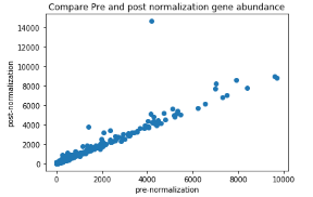
On investigating, I traced the issue down to the use of geometric mean of avgTxLength. I only knocked out one of the transcripts to demonstrate the problem, not because of any biological relevance. Hopefully the example above makes the issue clearer.
There is no issue with tximport's calculation of avgTxLength. The problem arises when the geometric mean of these average lengths is taken. The whole issue can be avoided (and the weighted average effective transcript lengths utilized) if the txCounts are divided by txLengths before summing into genes.
Please could you confirm or refute my example here?
Thanks, Mark
This is not a bug, this is the tximport method. The counts are scaled up for short genes and down for long genes (where short and long refer to the weighted average of effective transcript length, see tximport publication Supplemental Method Section 4 for details, which follows the algebra of the Cuffdiff2 paper).
If the isoform proportion estimates are correct then the counts should be scaled --> my point (2) above.
ah... thank you, I will study the paper.
Hi Michael, thanks for the reference to the paper. I have read the relevant section.
In defining transcript lengths it says:
For a single sample this would be:
Here we sum the product of txAbundance and txLength for each of the transcripts, i.e. it is summed over the transcripts of the gene.
The current implementation in DESeq2 replaces the vector with a single scalar value per gene, the avgTxLength.
It appears that for notational simplicity the paper uses the same effective length for each transcript across all samples, the mean of these sample effective lengths is implied. I assume that if we were to use sample specific effective lengths the equation would be:
again a vector, but here we would not be averaging transcript effective lengths across samples but would simply use the vector of effective lengths as provided.
To follow up on my examples, when effectiveLength is used as a vector the resulting gene expression counts make sense. In the contrived example the resulting gene expression shows a 10x difference as implied by the data. In the real world example using ENSG00000069275.12 again the resulting gene expression now also makes sense as implied by the counts.
I should also add that for the vast majority of genes this issue does not show up, as seen in the graph above. Generally the difference would go unnoticed.
No, that's not correct. The denominator (
sum_t' theta_{t'a} bar{l}_{t'a}) is theavgTxLength.The paper notation doesn't deal with multiple samples, but derives the offset that corrects the LFC for two samples. It generalizes to multiple samples.
DESeq2 with tximport-derived
avgTxLengthis correcting the vector of sample counts for a given gene by a vector of effective transcript lengths across samples, these are just centered on 1 (by dividing out the geometric mean) so that the scaled ("normalized") counts are close to the original counts. I don't follow when you say "when effectiveLength is used as a vector". For a given gene, the effective length correction is a vector across samples.Ah, thanks, the bar over the $l$ threw me off. I had interpreted that as an average taken in the algorithm thinking it was the average of all the Salmon EffectiveLengths for this transcript (or averageTxLength), but now I assume the bar simply indicates that the EffectiveLength is essentially an average produced upstream by Salmon.
so: $\sum_t{\theta_{t'a}\bar l_{t'a}}$ is the averageTxLength.
produced in tximport by:
So I'm clear on the tximport part, thank you for your patience.
What was throwing me off with
estimateSizeFactors.DESeqDataSetwas that after this I was retrieving the normalized counts withcounts(dds, normalized=TRUE)and then checking what the normalization had done to the data pre and post normalization by re-estimating abundance for the genes. I was taking:This caused the outlier in the identified gene. What I missed, is that since the normalization has factored in the geometric mean of avgTxLengths, the correct recalculation of abundance would be:
With this fix pre and post normalization abundance are now very similar and I have no outliers. Thank you for your help!
You're welcome!