Hello,

I am adapting limma to analyse colony-based fitness data in yeast (i.e. https://en.wikipedia.org/wiki/Synthetic_genetic_array).

For this, I am using arrayWeights() to calculate weights for each plate, and duplicateCorrelation() to take care of the technical replicates (where each yeast strain is grown multiple times next to each other).

After running the linear model using lmFit(), I need to calculate the prediction variance for each fitted value. In the case of a standard linear model constructed using lm(), this could be done using predict.lm(object, se.fit=TRUE).

However, such methods are not defined for MArrayLM objects from limma. I know that the fitted values themselves can be easily calculated:

fitted <- coef(object) %*% t(design)

To calculate the variance of each fitted value (prediction variance), I have adapted the approach outlined in this post: https://stackoverflow.com/questions/39337862/linear-model-with-lm-how-to-get-prediction-variance-of-sum-of-predicted-value/39338512#39338512

I have adapted it to deal with NAs (which includes using a different QR decomposition for each model) and adjusting the way that the residual variance is calculated to incorporate weights.

In the case that there are no technical replicates, this gives the following code, where object is the matrix of fitness values being modelled, design is the design matrix, and qrList is a list of QR decompositions - one for each linear model fitted. Note that for simplicity I am only predicting values for the first gene in this code:

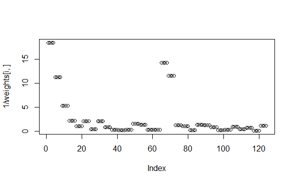
#Calclulate array weights
aw <- arrayWeights(object, design=design)
weights <- asMatrixWeights(aw, dim(object))

#Fit model
fit <- lmFit(object, design=design, weights=weights)

##Predict values according to model
coefs <- coef(fit)
coefs[is.na(coefs)] <- 0
predicted <- coefs %*% t(design)
predicted[is.na(object)] <- NA

##Calculate residuals
residuals <- object - predicted

#Calculate variance of fitted values for ith gene
i <- 1

#Get missing values
missing <- is.na(object[i,])

##complete variance-covariance matrix
QR <- qrList[[i]]   ## qr object of fitted model
piv <- QR$pivot     ## pivoting index
r <- QR$rank  
B <- forwardsolve(t(QR$qr), t(design[!missing, piv]), r)

## residual variance
#sig2 <- c(crossprod(residuals[i,])) / fit$df.residual[i]
sig2 <- c(crossprod((sqrt(weights[i,]) * residuals[i,])[!missing])) / fit$df.residual[i]

## return point-wise prediction variance
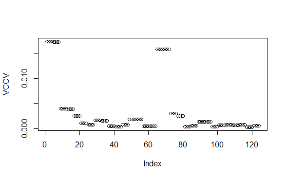
VCOV <- rep(NA, ncol(object))
VCOV[!missing] <- colSums(B ^ 2) * sig2

This code works and will give the same variance predictions as predict.lm(object, se.fit=TRUE) if I were to run a weighted linear model on the first gene using lm().

However, things become more complicated when I incorporate duplicateCorrelation() into my analysis as follows. Note that I have also used unwrapdups() to re-size object and weights, and I also re-size design:

#Calclulate array weights
aw <- arrayWeights(object, design=design)
weights <- asMatrixWeights(aw, dim(object))

#Calculate consensus correlation
dupcor <- duplicateCorrelation(myHDA, design=design, weights=aw)

#Fit model
#fit <- lmFit(object, design=design, weights=weights)
fit <- lmFit(object, design=design, correlation=dupcor$consensus.correlation, weights=weights)

#Get number of replicates and spacing
ndups <- unique(table(rownames(object)))
spacing <- 1

#Re-size to unwrap technical replicates
if(ndups > 1) {
  object <- limma::unwrapdups(object, ndups=ndups, spacing=spacing)
  weights <- limma::unwrapdups(weights, ndups=ndups, spacing=spacing)
  design <- design %x% rep(1, ndups)
}

##Predict values according to model
coefs <- coef(fit)
coefs[is.na(coefs)] <- 0
predicted <- coefs %*% t(design)
predicted[is.na(object)] <- NA

##Calculate residuals
residuals <- object - predicted

#Calculate variance of fitted values for ith gene
i <- 1

#Get missing values
missing <- is.na(object[i,])

##complete variance-covariance matrix
QR <- qrList[[i]]   ## qr object of fitted model
piv <- QR$pivot     ## pivoting index
r <- QR$rank  
B <- forwardsolve(t(QR$qr), t(design[!missing, piv]), r)

## residual variance
#sig2 <- c(crossprod(residuals[i,])) / fit$df.residual[i]
sig2 <- c(crossprod((sqrt(weights[i,]) * residuals[i,])[!missing])) / fit$df.residual[i]

## return point-wise prediction variance
VCOV <- rep(NA, ncol(object))
VCOV[!missing] <- colSums(B ^ 2) * sig2

This code will still provide variance estimates, but I think they are wrong. When I include duplicateCorrelation() in my pipeline, I noticed that the residual variance which I calculate, sig2, is not the same as the residual variance which comes from limma, fit$sigma[i]^2. This is not really surprising to me, although fixing it is beyond my understanding. Obviously, if I were only concerned with the residual variance, I could just use the values from limma, fit$sigma^2. However, I suspect that there may be other things going wrong because I am not taking the consensus correlation into account - perhaps calculation of the variance-covariance matrix?

So my question is this:

How do I adapt my code to account for the correlation between replicate spots when calculating the prediction variance of the fitted values?

Thank you in advance for any assistance.

Best wishes,

John

It you have computed the QR decomposition correctly for each gene, then computing the variances of the fitted values is easy. However you do need to have run eBayes, for example:

fit <- eBayes(fit)

You obviously cannot compute limma variances if you don't do the empirical Bayes calculations.

To compute the vector of estimated variances for the fitted-values for the ith gene:

Var <- hat( qrList[[i]] ) * fit$s2.post[i]

The computation is exactly the same whether you have used duplicateCorrelation or not, since the correlation is already incorporated into the QR decomposition.

The calculations from stackoverflow are unnecessary and are not entirely correct in the limma context.