Hello Jianhong,
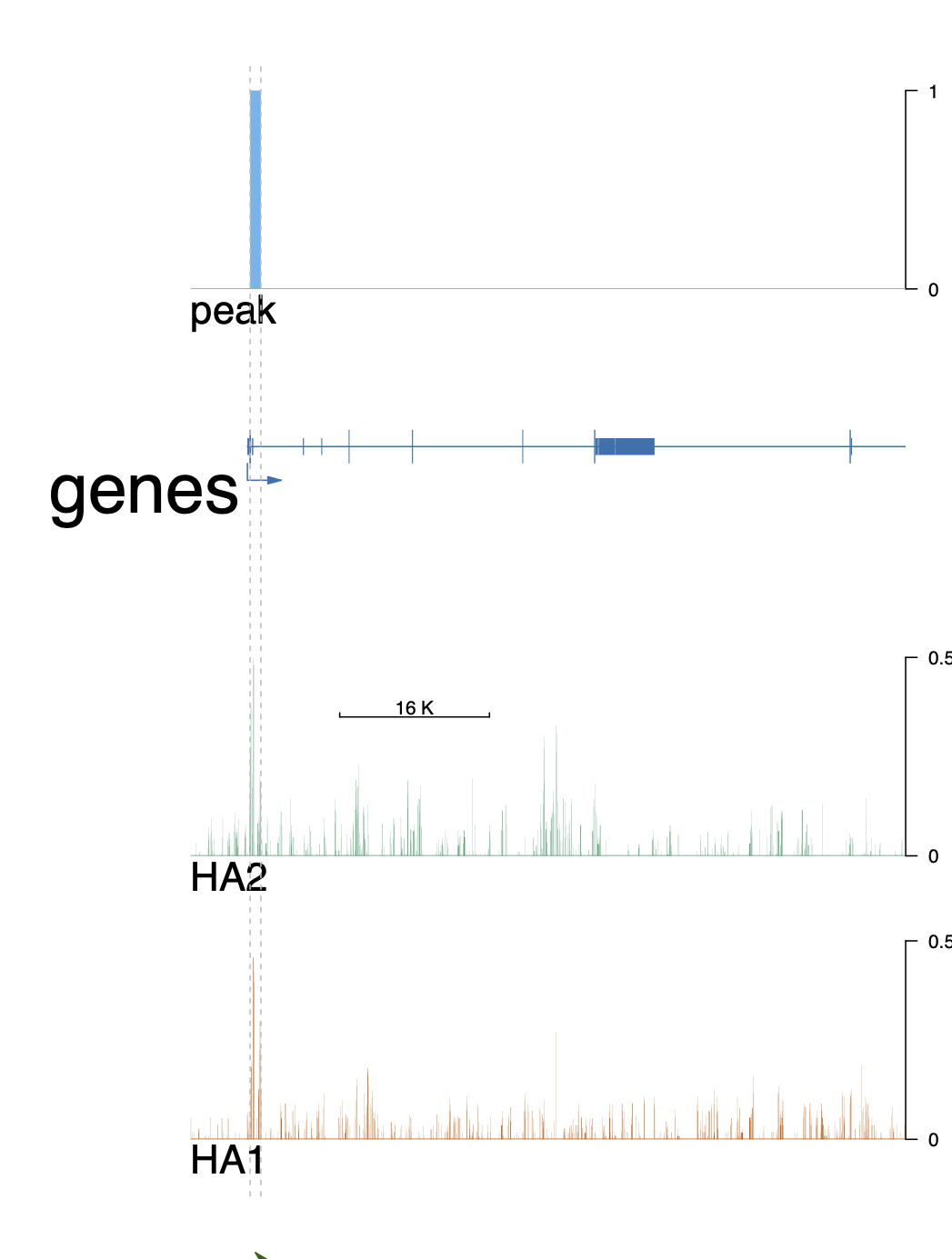
I intended to create trackView on ChIPSeq data align with the peak. I did not find a function in trackViewer to import peak.narrowPeak file, so I did the following
library(GenomicRanges)
peaks.gr <- parse2GRanges("chr9:69035856-69037005:+")
values(peaks.gr) <- DataFrame(score = c(1))
peak <- new("track", dat = trackViewer:::orderedGR(peaks.gr), type = "data", format = "BED")
Then I performed plotting, however, the peaks are not shown as what I intended, which is similar to an IGV peak visualization, or the exon visualization in trackViewer.
Is there a way to visualize peaks easily in trackViewer, e.g. a function to import bed/narrowPeak/broadPeak files?
Thanks a lot!!
optSty <- optimizeStyle(trackList(HA1, HA2, genes, peak), theme="safe")
trackList <- optSty$tracks
viewerStyle <- optSty$style

setTrackViewerStyleParam(viewerStyle, "margin", c(.05, .2, .05, .05)) #bottom, left, top and right margin.
setTrackXscaleParam(trackList[[2]], "draw", TRUE)
setTrackXscaleParam(trackList[[2]], "gp", list(cex=0.8))
# setTrackXscaleParam(trackList[[2]], attr="position",
#                     value=list(x=69035856, y=2, label=1000))
setTrackViewerStyleParam(viewerStyle, "xaxis", FALSE) # disable x ticks
setTrackStyleParam(trackList[[1]], "ylim", c(0, 0.5))
setTrackStyleParam(trackList[[2]], "ylim", c(0, 0.5))


vp <- viewTracks(trackList,
                 gr=gr, viewerStyle=viewerStyle,
                 autoOptimizeStyle=TRUE)

addGuideLine(c(69035856, 69037005), vp=vp) #peak1
addArrowMark(list(x=(69035856 + 69037005)/2,
                  y=2), # 2 means track 2 from the bottom.
             label="peak",
             col="darkgreen",
             vp=vp)


Looks much nicer now, thanks!!!
I used method2