Entering edit mode

Hi,
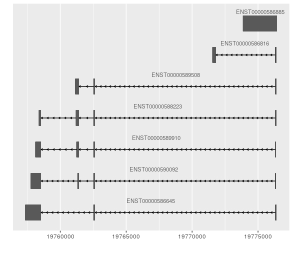
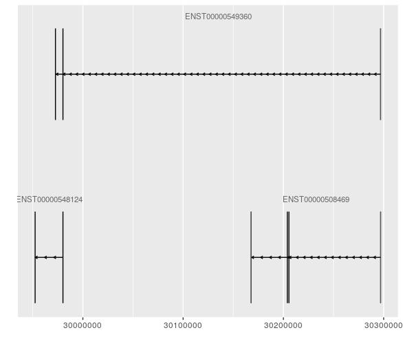
If there a way to produce uniformly sized gene models regardless of the number of transcripts? I have attached examples of a gene with two transcripts and another with a few.
Thanks
library(ggbio)
library(EnsDb.Hsapiens.v92)

ensdb <- EnsDb.Hsapiens.v92

autoplot(ensdb, GeneIdFilter("MyENSG")) #, names.expr = "gene_id")

R version 4.1.1 (2021-08-10)
Platform: x86_64-pc-linux-gnu (64-bit)
Running under: Ubuntu 18.04.5 LTS

Matrix products: default
BLAS:   /usr/lib/x86_64-linux-gnu/blas/libblas.so.3.7.1
LAPACK: /usr/lib/x86_64-linux-gnu/lapack/liblapack.so.3.7.1

locale:
 [1] LC_CTYPE=en_US.UTF-8       LC_NUMERIC=C               LC_TIME=en_US.UTF-8
 [4] LC_COLLATE=en_US.UTF-8     LC_MONETARY=en_US.UTF-8    LC_MESSAGES=en_US.UTF-8
 [7] LC_PAPER=en_US.UTF-8       LC_NAME=C                  LC_ADDRESS=C
[10] LC_TELEPHONE=C             LC_MEASUREMENT=en_US.UTF-8 LC_IDENTIFICATION=C

attached base packages:
[1] parallel  stats4    stats     graphics  grDevices utils     datasets  methods   base

other attached packages:
 [1] EnsDb.Hsapiens.v92_0.99.12  ensembldb_2.16.4            AnnotationFilter_1.16.0
 [4] GenomicFeatures_1.44.2      AnnotationDbi_1.54.1        ggbio_1.40.0
 [7] plyr_1.8.6                  rstatix_0.7.0               ggpubr_0.4.0
[10] viridis_0.6.2               viridisLite_0.4.0           ggplot2_3.3.5
[13] DESeq2_1.32.0               SummarizedExperiment_1.22.0 Biobase_2.52.0
[16] MatrixGenerics_1.4.3        matrixStats_0.61.0          GenomicRanges_1.44.0
[19] GenomeInfoDb_1.28.4         IRanges_2.26.0              S4Vectors_0.30.2
[22] BiocGenerics_0.38.0         data.table_1.14.2           reshape_0.8.8
[25] pheatmap_1.0.12             tidyr_1.1.4                 dplyr_1.0.7

loaded via a namespace (and not attached):
  [1] readxl_1.3.1             backports_1.4.1          Hmisc_4.6-0
  [4] BiocFileCache_2.0.0      lazyeval_0.2.2           splines_4.1.1
  [7] BiocParallel_1.26.2      digest_0.6.29            htmltools_0.5.2
 [10] fansi_1.0.2              magrittr_2.0.1           checkmate_2.0.0
 [13] memoise_2.0.1            BSgenome_1.60.0          cluster_2.1.2
 [16] openxlsx_4.2.5           Biostrings_2.60.2        annotate_1.70.0
 [19] prettyunits_1.1.1        jpeg_0.1-9               colorspace_2.0-2
 [22] blob_1.2.2               rappdirs_0.3.3           haven_2.4.3
 [25] xfun_0.29                crayon_1.4.2             RCurl_1.98-1.5
 [28] graph_1.70.0             genefilter_1.74.1        survival_3.2-13
 [31] VariantAnnotation_1.38.0 glue_1.6.0               gtable_0.3.0
 [34] zlibbioc_1.38.0          XVector_0.32.0           DelayedArray_0.18.0
 [37] car_3.0-12               abind_1.4-5              scales_1.1.1
 [40] DBI_1.1.2                GGally_2.1.2             Rcpp_1.0.8
 [43] xtable_1.8-4             progress_1.2.2           htmlTable_2.4.0
 [46] foreign_0.8-82           bit_4.0.4                OrganismDbi_1.34.0
 [49] Formula_1.2-4            htmlwidgets_1.5.4        httr_1.4.2
 [52] RColorBrewer_1.1-2       ellipsis_0.3.2           pkgconfig_2.0.3
 [55] XML_3.99-0.8             farver_2.1.0             nnet_7.3-17
 [58] dbplyr_2.1.1             locfit_1.5-9.4           utf8_1.2.2
 [61] tidyselect_1.1.1         labeling_0.4.2           rlang_0.4.12
 [64] reshape2_1.4.4           munsell_0.5.0            cellranger_1.1.0
 [67] tools_4.1.1              cachem_1.0.6             cli_3.1.0
 [70] generics_0.1.1           RSQLite_2.2.9            broom_0.7.11
 [73] stringr_1.4.0            fastmap_1.1.0            yaml_2.2.1
 [76] knitr_1.37               bit64_4.0.5              zip_2.2.0
 [79] purrr_0.3.4              KEGGREST_1.32.0          RBGL_1.68.0
 [82] xml2_1.3.3               biomaRt_2.48.3           compiler_4.1.1
 [85] rstudioapi_0.13          filelock_1.0.2           curl_4.3.2
 [88] png_0.1-7                ggsignif_0.6.3           tibble_3.1.6
 [91] geneplotter_1.70.0       stringi_1.7.6            forcats_0.5.1
 [94] lattice_0.20-44          ProtGenerics_1.24.0      Matrix_1.4-0
 [97] vctrs_0.3.8              pillar_1.6.4             lifecycle_1.0.1
[100] BiocManager_1.30.16      bitops_1.0-7             rtracklayer_1.52.1
[103] R6_2.5.1                 BiocIO_1.2.0             latticeExtra_0.6-29
[106] gridExtra_2.3            rio_0.5.29               dichromat_2.0-0
[109] assertthat_0.2.1         rjson_0.2.21             withr_2.4.3
[112] GenomicAlignments_1.28.0 Rsamtools_2.8.0          GenomeInfoDbData_1.2.6
[115] hms_1.1.1                grid_4.1.1               rpart_4.1-15
[118] carData_3.0-5            biovizBase_1.40.0        base64enc_0.1-3
[121] restfulr_0.0.13

Hi James, Thanks for the response! I found the chunk you are referring to, which would allow multiple tracks to be plotted and the height of each track specified. However if the genes do not overlap (may not even be on the same chromosome), but I am still interested in producing uniform gene model sizes for multiple genes, and the axis on the bottom would only be relevant for one of the genes I believe.
I am wondering maybe I can use the
heightsargument for a single graph? When I have added itautoplotseems to ignore the argument..I tried some workaround, displaying the same gene on both tracks and playing with the
heightsbut I still can't get the gene model to be the same size as it is still dependent on the number of transcripts displayed...OK, maybe I don't understand at all. From your original post I thought you wanted a single representative 'gene' rather than all the transcripts, which is what this is doing:
In particular the code for
p2.I am still assuming that's what you mean, although saying you want the 'gene model to be the same size' is not clear at all. What does 'size' mean in that context?
Hi James,
Sorry if I was unclear. I am referring to the height of the model itself, strictly speaking visualization. For publication I would like to represent some genes side by side, yet these genes have different number of transcripts, so without resizing manually each image I want to know if I can control the actual output of the heights of the gene models/transcripts so that the package doesn't fill the white space i.e. make the transcripts larger in size when there are only a few.
I hope that is clearer.
Thanks
Ah, I get it. You want the vertical height of the exons to be the same, regardless of the number of transcripts. That might be difficult to do and have it look reasonable. You can either keep the vertical height of the plots the same, in which case there would be an excess of empty space above the transcripts in the plot with fewer transcripts. Alternatively, you could shrink the vertical height of the plots to reflect the number of transcripts, in which case your plots would be of different sizes which might be a bit weird as well.
Anyway, if you are planning to use this in a publication you will need to output the plots anyway. You might play around with the size of the plot, reducing or increasing the vertical height in order to affect the resulting picture. In other words, something like
And the height of the first plot would be half the height of the second. In which case the exons should be +/- the same height?
Thanks, I'll keep working on it because the
png("two_transcripts.ong", 240)still looks a bit weird...thanks though!