
Hi,
I am relatively new to bioinformatics, but so far both the paper and the vignette have been very clear. However I still have a question since I am using the DESeq2 package for data other than bulk RNA-seq data.
I am trying to use the DESeq2 package for analysis of bulk methylation sequencing data. With the mouse model I am using methylation should correlate to RNA expression upon administration of doxycycline. So I have samples that were not induced by doxycycline (-dox) and thus have very little methylation (only background) and samples that do contain methylation (correlating to RNA expression). Some samples have more methylation than other due to the nature of the experiment.
What I am trying to understand is if my data fits the 'assumptions' and the analysis pipeline of the DESeq2 package, since I might have more 0 counts in my -dox samples and higher counts in the other samples and this should also stay this way to a certain extent.
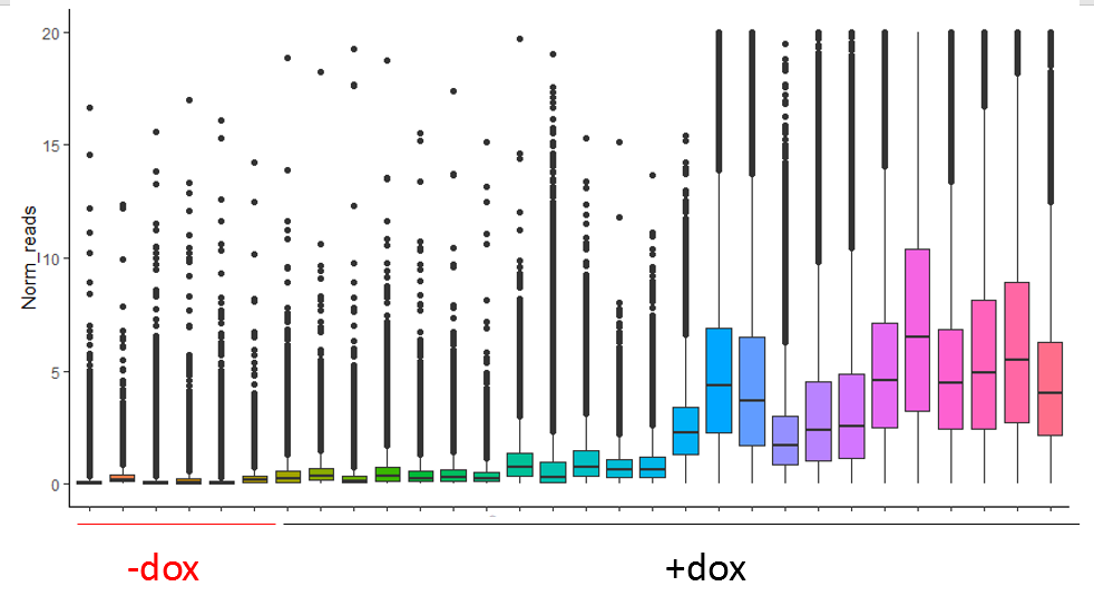
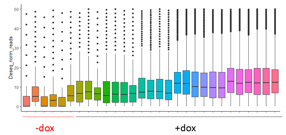
So far the DESeq2 package seems to work quite well for my data, and even after normalization with size factors estimated by DESeq2 itself my -dox samples have lower counts than all the others. (upper image before normalization and lower after)
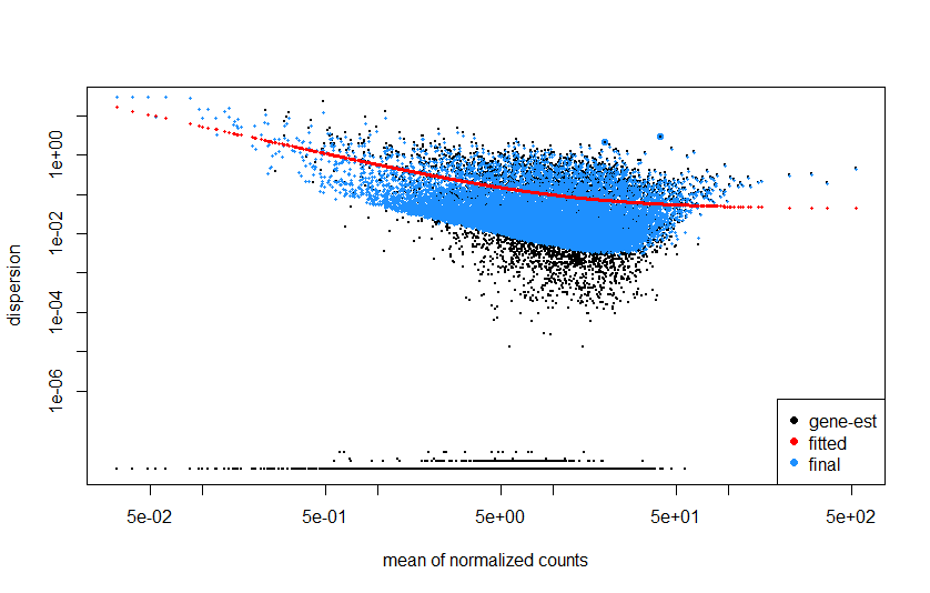
The next step for me was to look at the dispersion estimates plot. The plot I get is not very different from what I have seen in the examples (correct me if I am wrong). However I was wondering what the model does with the genes that have very low dispersion (so the two 'lines' at the bottom of the plot). If I understand it correctly these are genes with very low variability between samples so possibly housekeeping genes? But is the dispersion of these genes then also shrunken towards the red line?
Thank you a lot in advance!
Arina

Hi Michael,
Thank you for the fast reply! This explains it.
The complicated thing with my experiment is that the sequencing depth is actually equal across all samples. However, in the model that we use this specific type of methylation is lost over time (reads for other types of methylation are not shown here, but in the end add up to the same for all samples).
So within the +dox samples, the ones on the right have lost less methylation compared to the ones on the left, where at some point they become almost equal to the -dox samples. Still, I expect the -dox samples to only contain background (nonspecific methylation) and the +dox samples with low counts to contain highest counts on expressed genes but have lower values compared to +dox samples with high counts. This ofcourse in a way is the same as having less sequencing depth for these samples.
I tried to overcome this, by first running DESeq2 for comparison of -dox versus all other samples to find genes that are significantly upregulated above the negative control. Then I subset my original counts matrix for only these genes, remove the -dox samples and do the analysis again. This way the normalization seems to work better, than when I include the -dox samples.
I am not sure if i understand your solution correctly, but if I would do the down sampling I would lose information on highly expressed genes in the samples with 'higher sequencing depth' right? Or what do you exactly mean by anything that goes away?
Oh, I think then that this may not be well modeled with DESeq2. It sounds like you have global shifts, and it's difficult to account for that with how we do size factor scaling. If everything goes up in the counts that DESeq2 "sees", it's hard for the method to find what is an unchanging feature with no prior information.
Yes indeed, although this is only the case if the negative control samples are included. In this case the unchanging features are features that for some reason have high background. For all the other samples these should include both background and housekeeping genes.
Would it then make more sense to have my own size factors as an input based on the experimental design? So if I for example use a factor based on total counts of this methylation type in each sample? Could I then still do the dispersion estimate and the Wald test?
Doing that my normalization looks like this: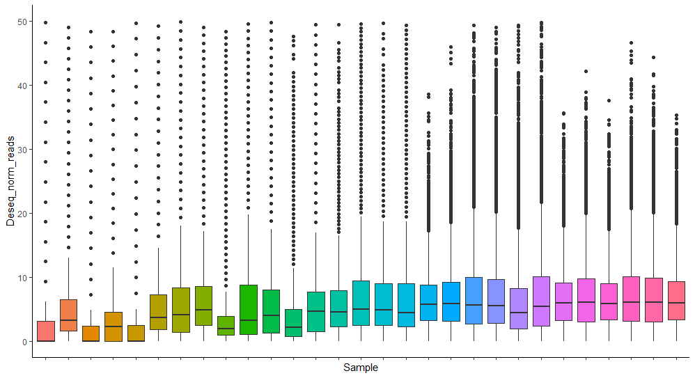
Yes you can in fact provide
controlGenesto tell DESeq2 which genes it should use for size factor estimationOr provide your own size factors (these must be positive, and centered near 1).