Hello Michael and the DESeq2 community,

In short. I have 38 samples of the same mouse tissue, half from line A and half from line B. I am interested in comparing subgroups within line A. I could just separate my dataset into two and perform DESeq only on line A samples, but I thought combining both would give me better estimations on sizeFactors and dispersions. However, if I put all samples into the same DDS, I couldn't add an important covariate.

My samples (colData)

38 mice. 17 in line A and 21 in line B. Each line consists of 3 litters (therefore 6 litters in total). In each litter, there can be both KO mice and WT mice. The 38 mice are also either trained or untrained. We are most interested in comparing trained line A KO to trained line A WT. But we also want to compare untrained line A KO to WT, trained line B KO to WT, and untrained line B KO to WT. To do this more easily, I combined "trained/untrained", "line A/B", and "KO/WT" into a single variable with 8 factors: "TAK", "TAW", "UAK", "UAW", "TBK", "TBW", "UBK", and "UBW".

In addition to these variables, we also recorded sex, body weight, tissues weight, RNA concentration, library concentration, death time, and time interval between training and death. All of these would be referred to as "all other covariates" in my codes below.

A design that worked ok

When I separated my data by the lines, I could, for example, perform DESeq on the 17 line A samples like this:

dds = DESeqDataSetFromMatrix(countData = cts_lineA, colData = coldata_lineA,
                                 design = ~ group + litter + (all other covariates))
dds = DESeq(dds, betaPrior = TRUE)
res = results(dds, contrast = list(c("groupTAK"), c("groupTAW")),
                listValues=c(1,-1), alpha = 0.05)
# I can also swap or combine groups to get the comparisons I want.
# The variable I care about -- "group", is not positioned at last, as suggested in most cases.
# From what I understand, since I'm explicit about which groups to compare in results(), this shouldn't matter.

I my case, I got ~40 genes that were significantly differentially expressed between TAK and TAW.

Problems with the approach

For some of these 40 genes, plotting the counts did not yield a visual impression corresponding to their p-values. For example:

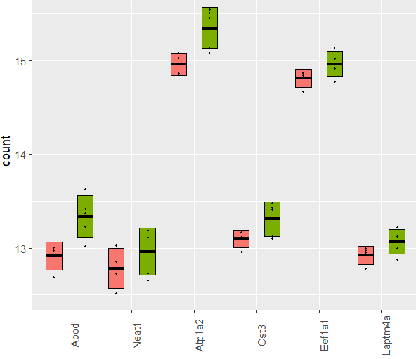
This plot shows limma-corrected (for all covariates), VST-transformed counts for genes that significantly went down (padj < 0.05) in Red (TAK) over Green (TAW). They are ordered according to padj from left (most significant) to right. While Apod has a l2fc of -0.84 and padj of 1.10E-05, Neat1 has a l2fc of -0.82 and padj of 1.10E-05. But the boxplot for Neat1 does not look very convincing. In addition to this, comparing 3 vs. 5 samples just feels risking getting false positive due to a few outliers.

Try incorporating information from lineB to better estimate sizeFactor and dispersion

To increase power of our comparison, my PI suggested me to incorporate information of line B. Unfortunately, I couldn't simple perform DESeq on all samples while using litter as a covariate due to Error in checkFullRank(modelMatrix):

dds = DESeqDataSetFromMatrix(countData = cts_all, colData = coldata_all,
                                 design = ~ group + litter + (all other covariates))

Error in checkFullRank(modelMatrix) : 
  the model matrix is not full rank, so the model cannot be fit as specified.
  One or more variables or interaction terms in the design formula are linear
  combinations of the others and must be removed.

We deemed litter as an indispensable covariate. Here is my tacky attempt to circumvent this problem:

# Obtaining sizeFactor and dispersion from all data
dds = DESeqDataSetFromMatrix(countData = cts_all, colData = coldata_all,
                                 design = ~ group + (all other covariates)) #no litter in design.
dds = estimateSizeFactors(dds)
dds = estimateDispersions(dds)

# Create a DDS with line A:
dds_line = DESeqDataSetFromMatrix(countData = cts_lineA, colData = coldata_lineA,
                                 design = ~ group + litter + (all other covariates)) #litter in design.
dds_line = estimateSizeFactors(dds_line)
dds_line = estimateDispersions(dds_line)

# Swap out the sizeFactors and dispersions
# Variable line_samples is the indices of lineA samples.
dds_line@colData@listData$sizeFactor = dds@colData@listData$sizeFactor[line_samples]
dds_line@assays@data@listData$mu = dds@assays@data@listData$mu[,line_samples]
dds_line@rowRanges@elementMetadata@listData = dds@rowRanges@elementMetadata@listData
dds_line = nbinomWaldTest(dds_line, betaPrior = TRUE)

In this case, sizeFactors from dds is basically the same as those from dds_line (~2% bigger to be precise.) However, dispersions from dds are nearly 10 times smaller than those from dds_line. Puzzlingly, with smaller dispersion, we lost all the DE genes.

My question

1. Is estimating sizeFactor and dispersion from as many samples as possible recommended? If so, is there a proper way to swap them in into a DDS?
2. Is VST transformation then limma batch correction the correct way to plot the gene counts?
3. Am I using betaPrior = TRUE correctly...?

Thank you for reading such a long post. Please let me know where I should clarify and if I should provide additional data/information. Thanks!