P-value inflation?
1
1
Entering edit mode
dsambo ▴ 10
@8678f435
Last seen 8 months ago
United States

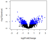
I ran DESeq2 (using default settings) comparing different groups (A vs B, with B having 1, 2, 3 subgroups). For the volcano plots below, red = adjusted pvalue < 0.1 and blue = pvalue < 0.05.

For the first comparison (A vs B1), there are no adjusted pvalue significant genes (expected).

enter image description here

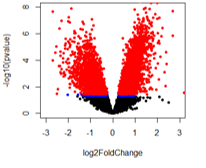
For the second comparison (A vs B2), there are a huge number of adjusted pvalue genes.

enter image description here

For the last comparison (A vs B3), it looks like there are pvalue significant genes that should also be adjusted pvalue significant but that doesn't seem to be the case.

enter image description here

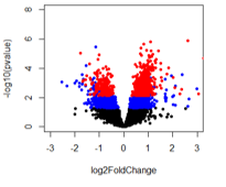
When comparing A vs B2 and A vs B3, it appears that genes are adjusted pvalue significant at lower pvalues than B2 compared to B3. I've looked at this with other adjusted p-value methods and get the same trend. Any ideas and what could be happened with A vs B2 to get what looks like pvalue inflation?

This is the code used to generate the volcano plots

#reset par
par(mfrow=c(1,1))
options(repr.plot.width=6, repr.plot.height=6)

# Make a basic volcano plot
with(res, plot(log2FoldChange, -log10(pvalue), pch=20, xlim=c(-3,3), ylim=c(0,8),
                xlab="log2FoldChange", ylab="-log10(p-value)", cex.axis = 1, cex.lab = 1))
with(subset(res, pvalue<.05), points(log2FoldChange, -log10(pvalue), pch=20, col="blue"))
with(subset(res, padj<.1), points(log2FoldChange, -log10(pvalue), pch=20, col="red"))
DESeq2 • 1.3k views
ADD COMMENT
1
Entering edit mode

The intensity of p-value adjustment, for most correction methods, trends with the number of comparisons being made. Do you happen to know the number of comparisons (tests) being performed for A vs B3 compared to A vs B2?

ADD REPLY
0
Entering edit mode

The number of comparisons appears to be the same for all (14,375), which I am basing of the DESeq2 summary "out of 14375 with nonzero total read count".

The number of pvalue < 0.05 genes is: A vs B1: 809; A vs B2: 5571; A vs B3: 2739

And the number of adjusted pvalue < 0.1 genes is: A vs B1: 0; A vs B2: 5077, A vs B3: 824

So out of the pvalue < 0.05 genes for A vs B2, 91% are also adjusted p-value significant. Seems off to me!

ADD REPLY
0
Entering edit mode
@james-w-macdonald-5106
Last seen 22 minutes ago
United States

You should show the code you used to make those volcano plots. Adjusted p-values are strictly monotonic, so I don't see how that plot reflects your results accurately. In other words, to adjust p-values (using BH I presume), the p-values are sorted in increasing order and then adjusted. The sorted p-values are strictly monotonic, as are the adjusted p-values. Your plot implies non-monotonicity of the adjusted p-values, which shouldn't be possible. The code for computing BH has been used by too many people too many times for any bugs to exist, so I think it's more likely that there is an error in the code you used to make those plots.

0
Entering edit mode

I've now included the code for the volcano plot! I did use BH for adjusted pvalue. Regardless of the plot, there is still a huge number of adjusted pvalue genes. The non-adjusted pvalues of genes that were signficant for that comparison are much higher (largest pvalue for A vs B2 is 0.03558 and the largest pvalue for A vs B3 is 0.007).

ADD REPLY
0
Entering edit mode

How did you generate your res object?

ADD REPLY
0
Entering edit mode

Particularly for the last two volcano plots, that is.

ADD REPLY
0
Entering edit mode

Please see below!

res2 <- results(dds, contrast=c("Response","Mid","Con"))
res3 <- results(dds, contrast=c("Response","Low","Con"))

#reset par
par(mfrow=c(1,1))
options(repr.plot.width=6, repr.plot.height=6)
# Make a basic volcano plot
with(res2, plot(log2FoldChange, -log10(pvalue), pch=20, xlim=c(-3,3), ylim=c(0,8),
                xlab="log2FoldChange", ylab="-log10(p-value)", cex.axis = 1, cex.lab = 1))
with(subset(res2, pvalue<.05), points(log2FoldChange, -log10(pvalue), pch=20, col="blue"))
with(subset(res2, padj<.1), points(log2FoldChange, -log10(pvalue), pch=20, col="red"))

#reset par
par(mfrow=c(1,1))
options(repr.plot.width=6, repr.plot.height=6)
# Make a basic volcano plot
with(res3, plot(log2FoldChange, -log10(pvalue), pch=20, xlim=c(-3,3), ylim=c(0,8),
                xlab="log2FoldChange", ylab="-log10(p-value)", cex.axis = 1, cex.lab = 1))
with(subset(res3, pvalue<.05), points(log2FoldChange, -log10(pvalue), pch=20, col="blue"))
with(subset(res3, padj<.1), points(log2FoldChange, -log10(pvalue), pch=20, col="red"))
ADD REPLY
0
Entering edit mode

What does design(dds) look like? And what about table(res3$pvalue < 0.05, res3$padj<0.1)?

ADD REPLY
0
Entering edit mode

Here are those lines!

design(dds) <- formula(~ Sex + Response)
dds <- DESeq(dds)

table(res3$pvalue < 0.05, res3$padj<0.1)

        FALSE TRUE
  FALSE  9122    0
  TRUE   1599  824
ADD REPLY
0
Entering edit mode

The table indicates that you have

  • 9122 genes with p>0.05 and FDR >0.1
  • 0 genes with p>0.05 and FDR<0.1
  • 1599 genes with p<0.05 and FDR>0.1
  • 825 genes with p<0.05 and FDR<0.1

In other words, the third volcano plot you show above doesn't reflect your results (as you don't have any FDR<0.1 where p>0.05).

ADD REPLY
0
Entering edit mode

Wouldn't the red points in the volcano plot 3 correspond to the 825 genes p<0.05 and FDR<0.1?

ADD REPLY
0
Entering edit mode

The issue with your third volcano plot is that your FDR values appear to be non-monotonic. In other words, you have blue points that have smaller p-values than other genes with significant FDR values (e.g., you have some FDR values that are not significant, based on p-values that are much smaller than other FDR values that arose from larger p-values). That shouldn't happen, which makes me think there is an error in your code somewhere. I guess really what I should have had you do is

> ord <- order(res3$pvalue)
> oFDR <- res3$padj[ord]
> all(oFDR == cummax(oFDR))

And if that is TRUE, then how you are coloring your points is wrong.

But your original question had to do with a comparison of your first and second volcano plots, where you have FDR values that are significant in the second plot, arising from p-values that are larger than those in the previous plot that weren't significant. This has to do with how BH is computed. Generally speaking, your unadjusted p-values have to be very close to achieving Bonferroni significance, or you won't have any significant genes. But if you do have one or more that meet Bonferroni, then you can have many more. Heuristically, what happens is the smallest p-value is adjusted using Bonferroni, and each successive p-value is adjusted by a fraction thereof. The main bit of code is this:

pmin(1, cummin(n/i * p[o]))[ro]

Where n is the number of genes, i is an indicator saying which p-value (in the ranked set of p-values from smallest to largest) we are adjusting, and p[0] is the p-value. So for the smallest p-value, the adjustment is n*p, which is Bonferroni. The next p-value's adjustment is (n/2)*p, or 'half Bonferroni'. The next is (n/3)*p and on and on. It's likely that you had no p-values close to Bonferroni in your first comparison, so no significant genes. But you had many that met Bonferroni in the second set, which is why all those genes meet FDR.

ADD REPLY

Login before adding your answer.

Traffic: 814 users visited in the last hour
Help About
FAQ
Access RSS
API
Stats

Use of this site constitutes acceptance of our User Agreement and Privacy Policy.

Powered by the version 2.3.6