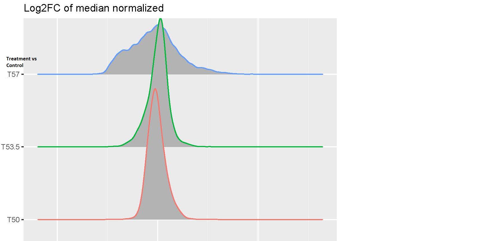
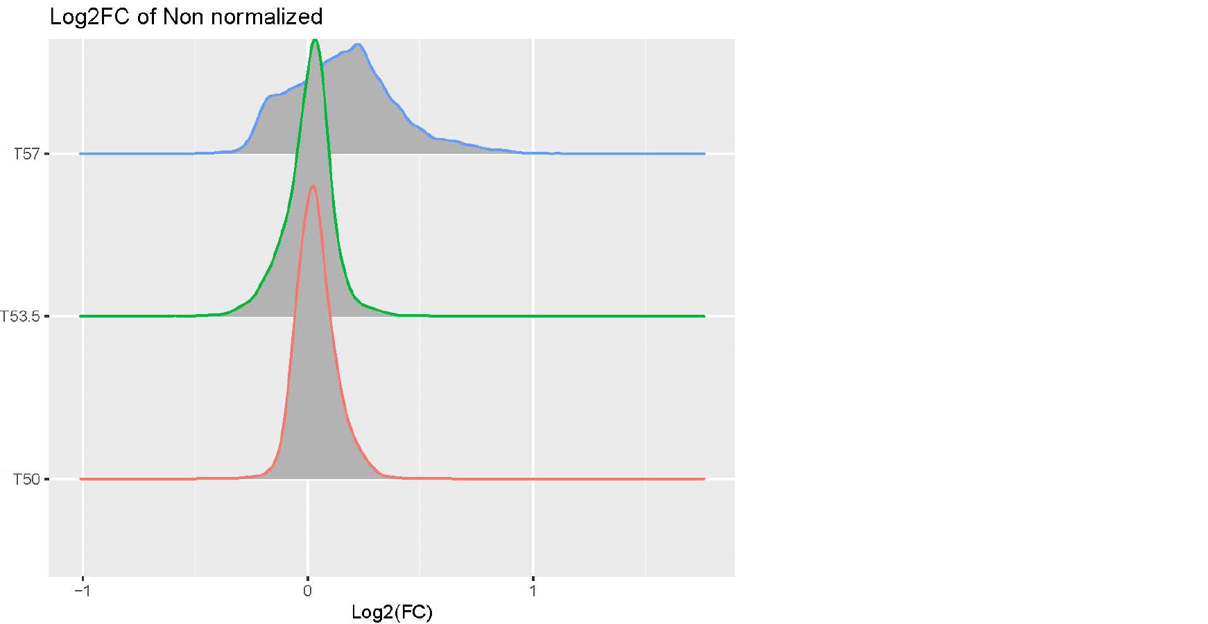
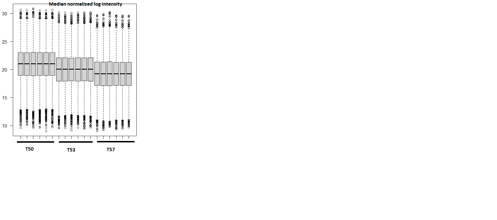
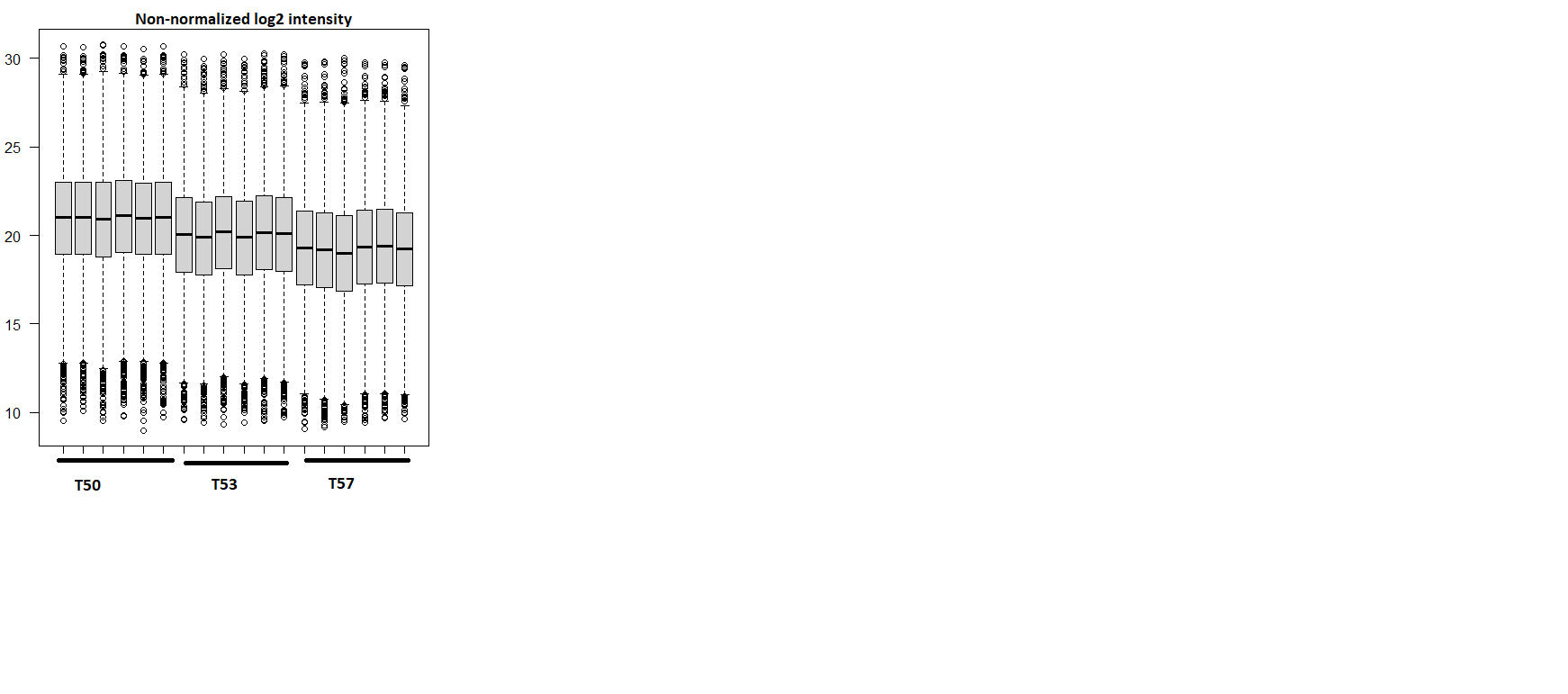
Hi, I am analyzing a data set with expression value of genes in the following conditions: cells with and without drug treatment at 3 different temperature(T): Control-T50 x3, Treatment-T53 x3, Control-T53 x3, Treatment-T53 x3, Control-T57 x3, Treatment-T57 x3. I processed the data using this pipeline: raw data > log2 transformation>median normalization for each temperature group (because temperature-dependent decrease of intensity is expected and needs to be preserved) >combine normalized samples back into one data table > limma DE analysis using one single factor matrix design (please see codes below). I then plotted log2FC of toptable output, but the logFC distribution of Treatment vs Control at T57 is very dispersed compared to other lower temperatures(see images attached). I've attached the logFC plots and intensity plots for non-normalized (raw) and median-normalized data set (please note the temperature-dependent decrease of intensity is expected).

My questions are (1) should I worry about this issue? (2) how can I fix this? I suspected the high variability of T57 samples but it doesn't seem so from the intensity plots. Any input would be appreciated, thanks very much. Please let me know if any other information I need to provide.

groups <- factor(groups, levels = c("ControlT50",
                                    "TreatmentT50",
                                    "ControlT53",
                                    "TreatmentT53",
                                    "ControlT57",
                                    "TreatmentT57"
))
design <- model.matrix(~ 0 + groups)
colnames(design) <- gsub("groups", "", colnames(design))
rownames(design) <- colnames(limma_df)

fitall <- limma::lmFit(limma_df, design)

meanint <- apply(limma_df, 1, function (x) {mean(x, na.rm =T)})
fitall$Amean <- meanint 

 contrast.matrix <- makeContrasts(TreatmentT50-ControlT50,
                                  TreatmentT53.5-ControlT53,
                                  TreatmentT57-ControlT57,
                                  levels=design) 


fitall <- limma::contrasts.fit(fitall, contrast.matrix)
fitall_eb <- limma::eBayes(fitall, trend = T)

toptable <- data.frame()
for (i in 1:length(colnames(fitall_eb))) {
  toptabdf <- limma::topTable(fitall_eb, coef = colnames(fitall_eb)[i],number = Inf, confint = T, adjust.method="BH")
  toptabdf <- toptabdf %>% mutate (Comparison = colnames(fitall_eb)[i]) 
  toptable <- rbind(toptable, toptabdf)

}

toptable %>%
         ggplot( aes(x = logFC, y = Comparison, color = Comparison ) ) +
         ggridges::geom_density_ridges()

 *limma* version: 3.65.2

# include your problematic code here with any corresponding output 
# please also include the results of running the following in an R session 

sessionInfo( R version 4.3.1 (2023-06-16 ucrt)
Platform: x86_64-w64-mingw32/x64 (64-bit)
Running under: Windows 10 x64 (build 17763))

There is no expectation for the distribution of the logFC values. Well, under the null they should be N(0, <sigma hat goes here>), but under the alternative, not so much. If you have lots of genes that are changing at the one temperature, then you should expect a larger spread. I mean that's what you are looking for, after all. But plotting the distribution of the logFC is not super useful anyway. Have you done PCA plots? How about MA plots?

That said, you seem to be doing some pretty non-standard things, although it's hard to say because you aren't being that forthcoming. You say it's gene expression data, but there are at least three different general classes of gene expression data that I can think of, and I would personally handle each one differently.

The rationale of a thermal protein profiling (TPP) experiment is that you will get large changes at the highest temperature and smaller or no changes at lower temperatures. So what you see is exactly what you would expect, is it not? I understand you are comparing treatment to control rather than comparing tempetures but the effects at high temperatures are always going to be variable. I am a bit puzzled what else you expected to see.

Analysis of TPP experiments is not straightforward and I can't tell you exactly how to do it. But I can make a few points:

• With just 3 temperatures, you can't do better than a single factor design. Your design matrix and DE analysis look ok in principle.
• You need some clever way to deal with missing values, if you are not doing so already. For a TPP experiment you can't just leave them as NA because they are not missing at random.
• I understand why you can't normalized globally, but I am still a bit uncomfortable about normalizing for each temperature group separately. Maybe that will be ok from comparing treatment to control but it will produce false positives if you compare temperatures for the same treatment. I would personally be inclined to leave unnormalized.

Your code seems complicated to me, partly because I don't use tidyverse. If you wanted to make histogram of logFC, you could simply use:

logFC <- fitall_eb$coef[,3]
hist(logFC, main="TreatmentT57-ControlT57")

It is strange to set fitall$Amean manually when limma already does this automatically.

This is no version 3.65.2 of limma. Perhaps you mean limma 3.56.2, which is the current release version.