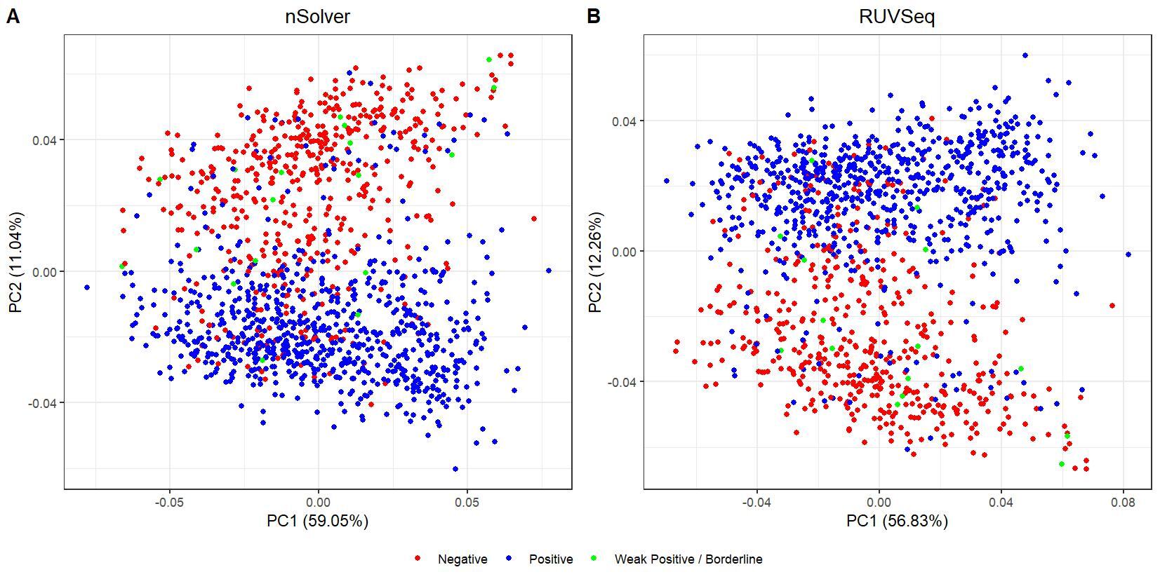
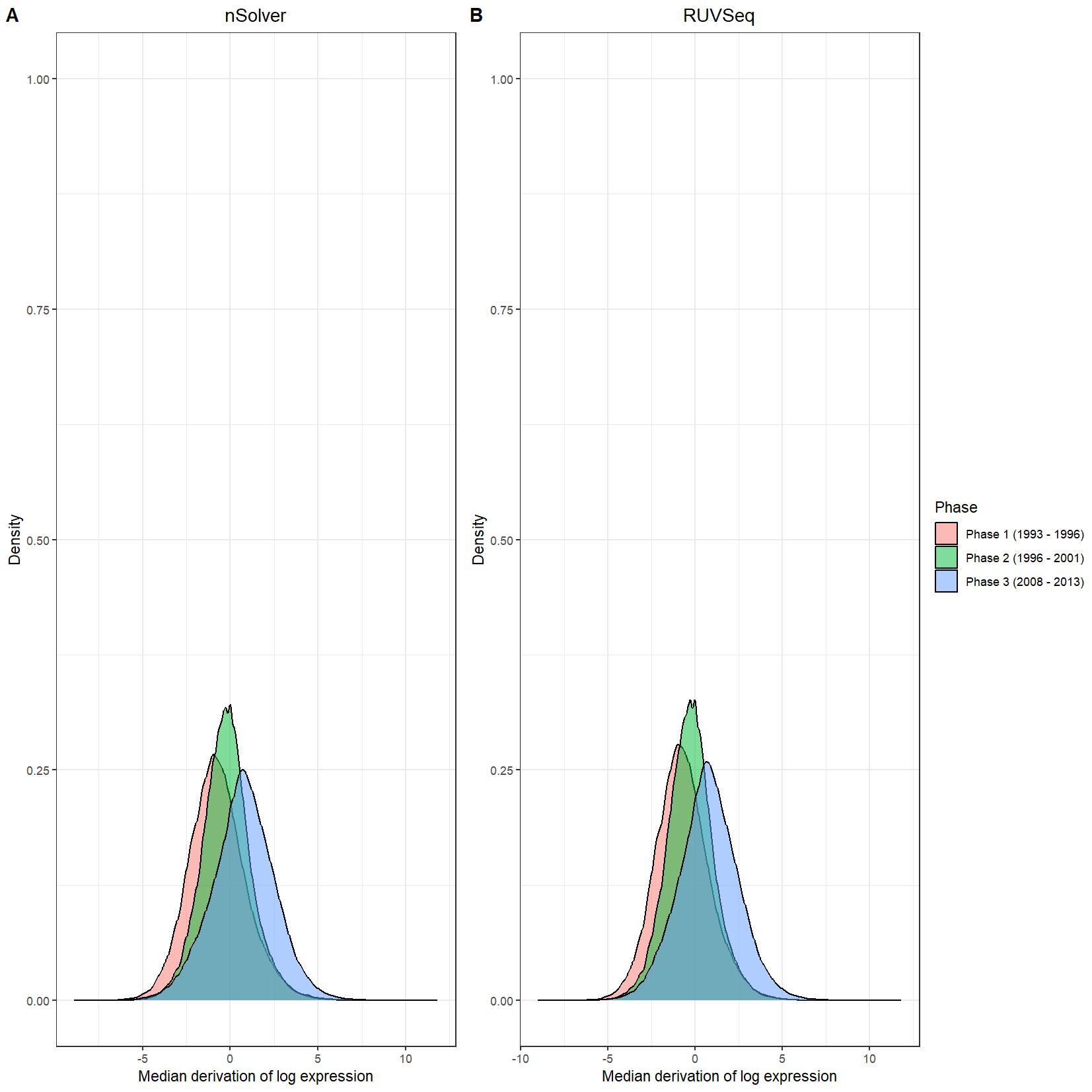
We have been trying to replicate part of the analysis of the paper titled 'An approach for normalization and quality control for NanoString RNA expression data' by Bhattacharya et al. To get a feeling for the effect of RUVseq normalization compared to nSolver normalization we tried to replicate some of the plots from Figure 2 using the CBCS data from GEO GSE148426 (which includes GSE148425 and GSE148418). At the moment, we are failing achieve similar PCA plots using the already normalized data in GEO. Most of the biological variance goes in PC2. Also, our silhouette plots and density plots differ a little. Could you be so kind to help us understand what we are doing wrong? You can find the code and images below. Thank you for your help!

######## LOAD OR INSTALL NECESSARY PACKAGES ########
library(nanostringr)
library(ggpubr)
library(tidyverse)
library(cluster)
library(ggplot2)
library(ggfortify)

######## DEFINE GLOBAL VARIABLES ########
NSOLVER.DATA.FOLDER <- "./GSE148418/" # Directory containing the RCC files downloaded from GEO
RUVSEQ.DATA.FOLDER <- "./GSE148425/" # Directory containing the RCC files downloaded from GEO
RESULTS.FOLDER <- "./Results/"
NSOLVER.ANNOTATION.FILE <- "./GSE148418/GSE148418_metadata.csv" # Annotation file generated from raw series matrix
RUVSEQ.ANNOTATION.FILE <- "./GSE148425/GSE148425_metadata.csv" # Annotation file generated from raw series matrix
PLOT.COLORS <- c("red", "blue", "green", "orange", "darkgreen", "black", "yellow", "pink")

# Read data
rcc_files_nsolver <- read_rcc(NSOLVER.DATA.FOLDER)
nsolver_dat <- rcc_files_nsolver$raw
rownames(nsolver_dat) <- nsolver_dat$Name
rcc_files_ruvseq <- read_rcc(RUVSEQ.DATA.FOLDER)
ruvseq_dat <- rcc_files_ruvseq$raw
rownames(ruvseq_dat) <- ruvseq_dat$Name
clin_lab_nsolver <- read.csv(NSOLVER.ANNOTATION.FILE) # Import Annotations
rownames(clin_lab_nsolver) <- paste(clin_lab_nsolver$Sample_geo_accession, clin_lab_nsolver$Sample_description, sep="_")
clin_lab_nsolver$Sample_characteristics_ch1 <- gsub("study phase: ", "", clin_lab_nsolver$Sample_characteristics_ch1)
clin_lab_nsolver$Sample_characteristics_ch1.2 <- gsub("estrogen receptor status: ", "", clin_lab_nsolver$Sample_characteristics_ch1.2)
clin_lab_ruvseq <- read.csv(RUVSEQ.ANNOTATION.FILE) # Import Annotations
rownames(clin_lab_ruvseq) <- paste(clin_lab_ruvseq$Sample_geo_accession, clin_lab_ruvseq$Sample_description, sep="_")
clin_lab_ruvseq$Sample_characteristics_ch1.1 <- gsub("study phase: ", "", clin_lab_ruvseq$Sample_characteristics_ch1.1)
clin_lab_ruvseq$Sample_characteristics_ch1.2 <- gsub("estrogen receptor status: ", "", clin_lab_ruvseq$Sample_characteristics_ch1.2)

# Log transform data
log_nsolver_dat <- log2(nsolver_dat[,-c(1:3)]+1)
log_ruvseq_dat <- log2(ruvseq_dat[,-c(1:3)]+1)

# Density plots log data
nsolver_medians <- apply(as.data.frame(log_nsolver_dat), 1, median)
nsolver_devs_from_median <- as.data.frame(log_nsolver_dat) - nsolver_medians
nsolver_devs_from_median_long <- gather(nsolver_devs_from_median, key = patient, value = value)
nsolver_devs_from_median_long$Phase <- clin_lab_nsolver[nsolver_devs_from_median_long$patient, 'Sample_characteristics_ch1']
ruvseq_medians <- apply(as.data.frame(log_ruvseq_dat), 1, median)
ruvseq_devs_from_median <- as.data.frame(log_ruvseq_dat) - ruvseq_medians
ruvseq_devs_from_median_long <- gather(ruvseq_devs_from_median, key = patient, value = value)
ruvseq_devs_from_median_long$Phase <- clin_lab_ruvseq[ruvseq_devs_from_median_long$patient, 'Sample_characteristics_ch1.1']

nsolver_density_plot <- ggplot(nsolver_devs_from_median_long, aes(x = value, fill = Phase)) +
    geom_density(alpha = 0.5) +
    scale_color_manual(values=PLOT.COLORS) +
    theme_bw() +
    labs(x = "Median derivation of log expression", y = "Density") +
    ggtitle("nSolver") +
    theme(plot.title = element_text(hjust = 0.5)) +
  scale_y_continuous(limits = c(0, 1))

ruvseq_density_plot <- ggplot(ruvseq_devs_from_median_long, aes(x = value, fill = Phase)) +
  geom_density(alpha = 0.5) +
  scale_color_manual(values=PLOT.COLORS) +
  theme_bw() +
  labs(x = "Median derivation of log expression", y = "Density") +
  ggtitle("RUVSeq") +
  theme(plot.title = element_text(hjust = 0.5))+
  scale_y_continuous(limits = c(0, 1))

jpeg(paste0(RESULTS.FOLDER, "Density_plots.jpeg"), units="cm", width=28, height=28, res=150)
ggarrange(nsolver_density_plot, ruvseq_density_plot, common.legend = TRUE, legend="right", labels = LETTERS[1:2])
dev.off()

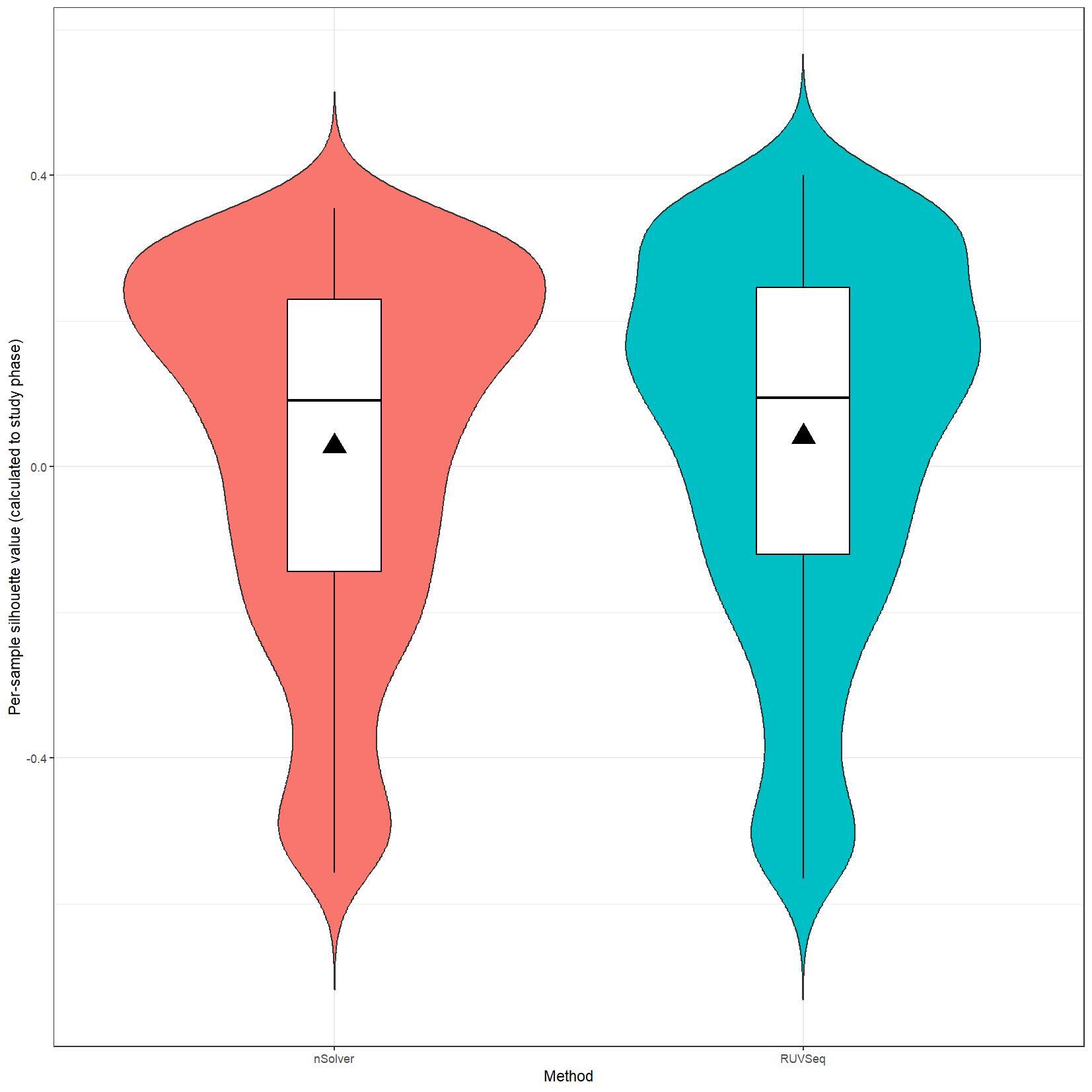
# Silhouette violin plots
clin_lab_nsolver$Silhouette.cluster <- clin_lab_nsolver$Sample_characteristics_ch1
clin_lab_nsolver <- clin_lab_nsolver %>% mutate(Silhouette.cluster = recode(Silhouette.cluster, "Phase 1 (1993 - 1996)" = 1, "Phase 2 (1996 - 2001)" = 2, "Phase 3 (2008 - 2013)" = 3))
nsolver_silhouette_vals <- silhouette(clin_lab_nsolver[colnames(nsolver_dat[,-c(1:3)]), 'Silhouette.cluster'], dist(t(log_nsolver_dat))^2)
clin_lab_ruvseq$Silhouette.cluster <- clin_lab_ruvseq$Sample_characteristics_ch1.1
clin_lab_ruvseq <- clin_lab_ruvseq %>% mutate(Silhouette.cluster = recode(Silhouette.cluster, "Phase 1 (1993 - 1996)" = 1, "Phase 2 (1996 - 2001)" = 2, "Phase 3 (2008-2013)" = 3))
ruvseq_silhouette_vals <- silhouette(clin_lab_ruvseq[colnames(ruvseq_dat[,-c(1:3)]), 'Silhouette.cluster'], dist(t(log_ruvseq_dat))^2)
silhouette_vals_df <- rbind(as.data.frame.matrix(nsolver_silhouette_vals), as.data.frame.matrix(ruvseq_silhouette_vals))
silhouette_vals_df$Method <- c(rep("nSolver", nrow(nsolver_silhouette_vals)), rep("RUVSeq", nrow(ruvseq_silhouette_vals)))

jpeg(paste0(RESULTS.FOLDER, "Silhouette_plots.jpeg"), units="cm", width=28, height=28, res=150)
ggplot(silhouette_vals_df, aes(x = Method, y = sil_width, fill = Method)) +
  geom_violin(trim=F) +
  geom_boxplot(width=0.2, color="black", fill="white") +
  stat_summary(fun.y=mean, geom="point", shape=17, size=6, fill="black") +
  scale_color_manual(values=PLOT.COLORS) +
  theme_bw() +
  theme(legend.position = "none") +
  labs(x = "Method", y = "Per-sample silhouette value (calculated to study phase)")
dev.off()

# PCA plots
pca_nsolver_dat <- log_nsolver_dat[,clin_lab_nsolver$Sample_characteristics_ch1.2 != "Unknown"] # remove samples with unknown subtype to make figure more clear
pca_ruvseq_dat <-log_ruvseq_dat[,clin_lab_ruvseq$Sample_characteristics_ch1.2 != "Unknown"]# remove samples with unknown subtype to make figure more clear
pca_nsolver <- prcomp(t(pca_nsolver_dat), scale. = F)
pca_plot_nsolver <- autoplot(pca_nsolver,
                 data = clin_lab_nsolver[clin_lab_nsolver$Sample_characteristics_ch1.2 != "Unknown",],
                 colour = "Sample_characteristics_ch1.2",
                 label = F) + scale_color_manual(values=PLOT.COLORS) + theme_bw() + ggtitle("nSolver") + theme(plot.title = element_text(hjust = 0.5), legend.title = element_blank())
pca_ruvseq <- prcomp(t(pca_ruvseq_dat), scale. = F)
pca_plot_ruvseq <- autoplot(pca_ruvseq,
                             data = clin_lab_ruvseq[clin_lab_ruvseq$Sample_characteristics_ch1.2 != "Unknown",],
                             colour = "Sample_characteristics_ch1.2",
                             label = F) + scale_color_manual(values=PLOT.COLORS) + theme_bw() + ggtitle("RUVSeq") + theme(plot.title = element_text(hjust = 0.5), legend.title = element_blank())
jpeg(paste0(RESULTS.FOLDER, "PCA_plots_estrogen_receptor_status.jpeg"), units="cm", width=28, height=14, res=150)
ggarrange(pca_plot_nsolver, pca_plot_ruvseq, common.legend = TRUE, legend="bottom", labels = c("A", "B"))
dev.off()

Can you pull out the first few expression values for patient 1 CBCS_N1 in your R session? Let's confirm that you've got the same data as we expect.

If I go to GEO I get:

# nSolver:
ID_REF  VALUE
ABAT    2.89
ABCB1   5.47
ABCC8   3.89

# RUV:
ID_REF  VALUE
ABAT    2.163217504
ABCB1   4.791834442
ABCC8   3.510253365