
Hello everybody,
I am analyzing a dataset of RNAseq data generated previously. Basically, the dataset is made of 3 conditions, with 4 biological replicates in each condition, and 2 technical replicates per biological condition (maybe the best choice, but the data is here...). I am observing massive LFC shrinkage (almost all genes LFC are shrinked to 0) in my analysis, even though the counts seems OK.
I first filter the counts using counts_data <- counts_data[which(rowSums(counts_data>=10) >= 8),], ending up with 15126 genes (that might be important?).
I create the dds object using dds <- DESeqDataSetFromMatrix(countData = counts_data, colData = metadata, design = ~Experimental_condition) and then do ddsColl <- collapseReplicates(dds, dds$Replicate, dds$Sample_name) to merge technical replicates, and proceed with the analysis normally:
contrast_exchange_vs_alone <- c("Experimental_condition", "E", "B")
res_exchange_vs_alone <- results(ddsColl, contrast=contrast_exchange_vs_alone, alpha = 0.05)
res_exchange_vs_alone_lfcshrink <- lfcShrink(ddsColl, coef="Experimental_condition_E_vs_B", res=res_exchange_vs_alone) #type='apeglm' default
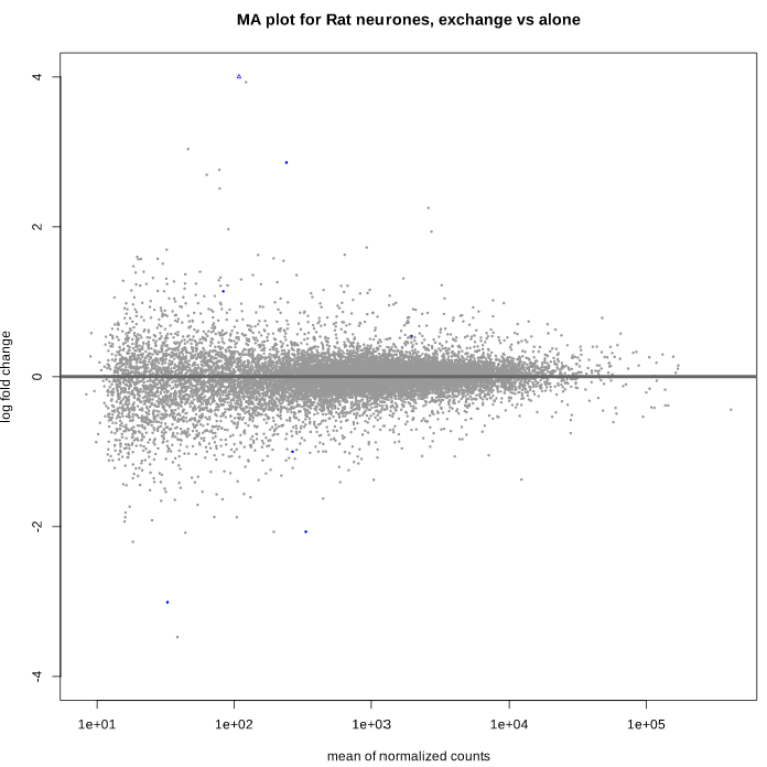
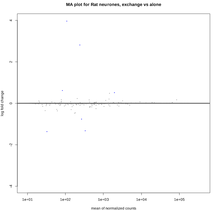
Here is the MA plot before shrinkage:
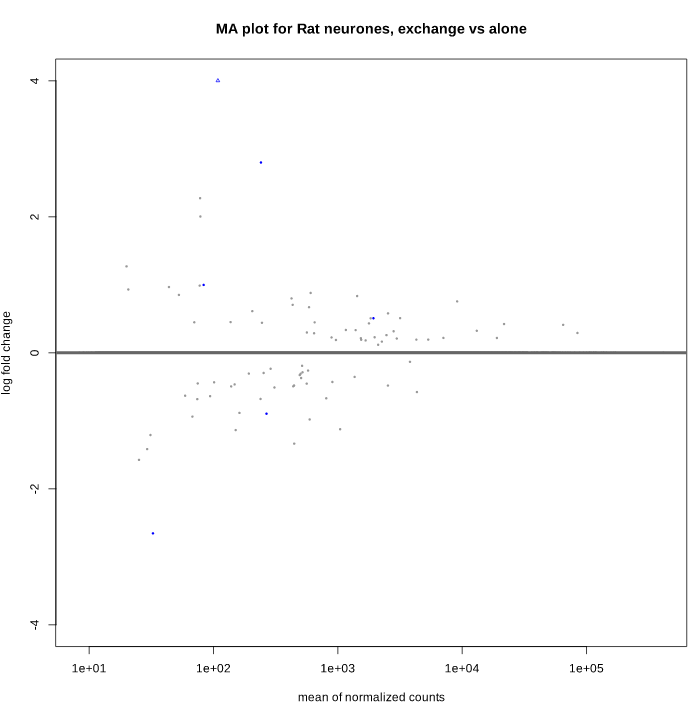
And after shrinkage (apeglm):
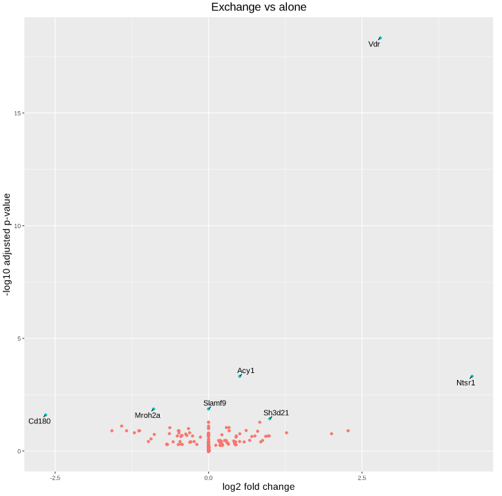
Here is the volcano plot after shrinkage:
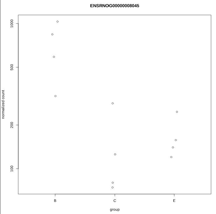
As you can see, some gene's LFC are heavily shifted towards 0. Let's take a closer look at gene ENSRNOG00000008045 (a.k.a Slamf9), here is the plotCounts for normalized counts:
Same gene, raw counts:
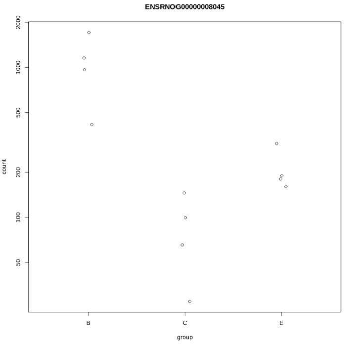
There is indeed some variability between replicates, but I am surprised that the LFC was shrinked to 0 for this gene. All counts are > 100 for the conditions under study ("E" and "B"). Do you have any clue why LFC shrink is so drastic, and what is going on in my analysis/dataset?
Thank you in advance for your help and insights,
Theo
Edit 1:
The MA plot looks similar with lfcShrink(type='ashr'):
I suspect something is off with the data but I have not been able to track it down...
> sessionInfo()
R version 4.3.2 (2023-10-31)
Platform: x86_64-conda-linux-gnu (64-bit)
Running under: Ubuntu 20.04.5 LTS

Matrix products: default
BLAS/LAPACK: /home/xxxx/miniconda3/envs/yyyy/lib/libopenblasp-r0.3.25.so;  LAPACK version 3.11.0

locale:
 [1] LC_CTYPE=C.UTF-8       LC_NUMERIC=C           LC_TIME=C.UTF-8
 [4] LC_COLLATE=C.UTF-8     LC_MONETARY=C.UTF-8    LC_MESSAGES=C.UTF-8
 [7] LC_PAPER=C.UTF-8       LC_NAME=C              LC_ADDRESS=C
[10] LC_TELEPHONE=C         LC_MEASUREMENT=C.UTF-8 LC_IDENTIFICATION=C

time zone: Europe/Paris
tzcode source: system (glibc)

attached base packages:
[1] grid      stats4    stats     graphics  grDevices utils     datasets
[8] methods   base

other attached packages:
 [1] org.Rn.eg.db_3.18.0         org.Hs.eg.db_3.18.0
 [3] Orthology.eg.db_3.18.0      AnnotationDbi_1.64.1
 [5] ggrepel_0.9.4               pheatmap_1.0.12
 [7] GGally_2.2.0                DEGreport_1.38.4
 [9] ggiraph_0.8.8               ggplot2_3.4.4
[11] DESeq2_1.42.0               SummarizedExperiment_1.32.0
[13] Biobase_2.62.0              MatrixGenerics_1.14.0
[15] matrixStats_1.2.0           GenomicRanges_1.54.1
[17] GenomeInfoDb_1.38.1         IRanges_2.36.0
[19] S4Vectors_0.40.2            BiocGenerics_0.48.1
[21] FactoMineR_2.9              BiocManager_1.30.22

loaded via a namespace (and not attached):
  [1] RColorBrewer_1.1-3          ggdendro_0.1.23
  [3] shape_1.4.6                 magrittr_2.0.3
  [5] estimability_1.4.1          farver_2.1.1
  [7] GlobalOptions_0.1.2         zlibbioc_1.48.0
  [9] vctrs_0.6.5                 memoise_2.0.1
 [11] RCurl_1.98-1.13             htmltools_0.5.7
 [13] S4Arrays_1.2.0              progress_1.2.3
 [15] broom_1.0.5                 SparseArray_1.2.2
 [17] htmlwidgets_1.6.4           plyr_1.8.9
 [19] emmeans_1.9.0               cachem_1.0.8
 [21] uuid_1.1-1                  lifecycle_1.0.4
 [23] iterators_1.0.14            pkgconfig_2.0.3
 [25] Matrix_1.6-4                R6_2.5.1
 [27] fastmap_1.1.1               GenomeInfoDbData_1.2.11
 [29] clue_0.3-65                 numDeriv_2016.8-1.1
 [31] digest_0.6.33               colorspace_2.1-0
 [33] reshape_0.8.9               RSQLite_2.3.4
 [35] labeling_0.4.3              fansi_1.0.6
 [37] mgcv_1.9-1                  httr_1.4.7
 [39] abind_1.4-5                 compiler_4.3.2
 [41] bit64_4.0.5                 withr_2.5.2
 [43] doParallel_1.0.17           ConsensusClusterPlus_1.66.0
 [45] backports_1.4.1             BiocParallel_1.36.0
 [47] viridis_0.6.4               DBI_1.2.0
 [49] psych_2.3.12                ggstats_0.5.1
 [51] dendextend_1.17.1           MASS_7.3-60
 [53] DelayedArray_0.28.0         rjson_0.2.21
 [55] scatterplot3d_0.3-44        flashClust_1.01-2
 [57] tools_4.3.2                 glue_1.6.2
 [59] nlme_3.1-164                cluster_2.1.6
 [61] generics_0.1.3              isoband_0.2.7
 [63] gtable_0.3.4                tidyr_1.3.0
 [65] hms_1.1.3                   utf8_1.2.4
 [67] XVector_0.42.0              foreach_1.5.2
 [69] pillar_1.9.0                stringr_1.5.1
 [71] emdbook_1.3.13              limma_3.58.1
 [73] splines_4.3.2               logging_0.10-108
 [75] circlize_0.4.15             dplyr_1.1.4
 [77] lattice_0.22-5              bit_4.0.5
 [79] tidyselect_1.2.0            ComplexHeatmap_2.18.0
 [81] locfit_1.5-9.8              Biostrings_2.70.1
 [83] knitr_1.45                  gridExtra_2.3
 [85] edgeR_4.0.2                 xfun_0.41
 [87] statmod_1.5.0               DT_0.31
 [89] stringi_1.8.3               codetools_0.2-19
 [91] bbmle_1.0.25.1              tibble_3.2.1
 [93] multcompView_0.1-9          cli_3.6.2
 [95] xtable_1.8-4                systemfonts_1.0.5
 [97] munsell_0.5.0               Rcpp_1.0.11
 [99] coda_0.19-4                 png_0.1-8
[101] bdsmatrix_1.3-6             parallel_4.3.2
[103] leaps_3.1                   blob_1.2.4
[105] prettyunits_1.2.0           bitops_1.0-7
[107] apeglm_1.24.0               viridisLite_0.4.2
[109] mvtnorm_1.2-4               scales_1.3.0
[111] purrr_1.0.2                 crayon_1.5.2
[113] GetoptLong_1.0.5            rlang_1.1.2
[115] cowplot_1.1.2               KEGGREST_1.42.0
[117] mnormt_2.1.1
