Divergent results using exact, glmLRT, and glmQLF tests in edgeR
1
0
Entering edit mode
Marianna ▴ 20
@7cc5052f
Last seen 16 days ago
Italy

Hi to everybody!

I'm analyzing an RNA-seq dataset (n=28; 1 factor, 4 variables: normal, SM, WS, WB) and I'm finding some unexpected results when comparing the three tests provided by the edgeR package: exact test, glmLRT, glmQLF.

Usually, as a preliminary exploratory analysis, I perform all the three tests mentioned above and the results are in agreement; the only thing that usually changes is the number of DEGs (Exact test>glmLRT>glmQLF). Assume for instance the following dataset: CTRL, conditionA and conditionB. If the condition A affects the gene expression more than the condition B, thus the output of the three tests will be consistent (all saying the condition A determines the most relevant effects).

With this new dataset, I did the exploratory analysis and the exact test and the glmLRT are in agreement (no, or small effects), while the glmQLF produces several DEGS in the conditions WS and WB. Below the results

DEGs with exact test

  • SM vs Normal: 4

  • WS vs Normal: 0

  • WB vs Normal: 0

DEGs with glmLRT

  • SM vs Normal: 6

  • WS vs Normal: 0

  • WB vs Normal: 0

DEGs with glmQLF

  • SM vs Normal: 0

  • WS vs Normal: 143

  • WB vs Normal: 125

Why this result is so divergent??? Which test is reliable? Suggestions are welcome!!

Below I copy the "simplified" code.

treat <-factor (targets$myopathies, levels =c("Normal","WS","WB","SM"))
myDGEList <- DGEList(counts= myCounts, group=treat)
design <- model.matrix(~0+treat)
keep<-filterByExpr(myDGEList, group=treat)
filter<- myDGEList[keep, , keep.lib.sizes=FALSE]
myDGEList.filtered.norm <- normLibSizes(filter, method="TMM")
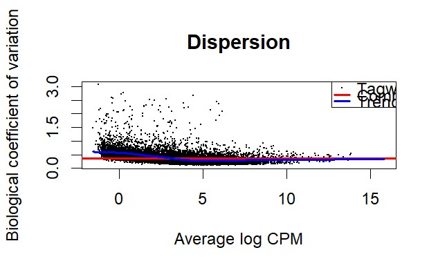
disp <- estimateDisp(myDGEList.filtered.norm, design, robust=TRUE)
### common disp: 0.128

dispersion

## exact test
exact.SM <- exactTest(disp, pair=c("Normal","SM"))

## LRT
fit_lrt<- glmFit(disp, design, robust=TRUE)
LRTtest.SM<- glmLRT(fit_lrt, contrast=my.contrasts [, "d42_SM"])

## QLF
fit_qlf<- glmQLFit(disp, design, robust=TRUE)
QLFtest.SM<- glmQLFTest(fit_qlf, contrast=my.contrasts [, "d42_SM"])

Thank you for your time and attention!

Marianna

edgeR • 612 views
ADD COMMENT
0
Entering edit mode

Which version of edgeR are you using? Please see the FAQ or the posting guide.

The code you show is incomplete because it does't explain the contrast that is being tested. You don't seem to be undertaking the same comparison for glmLRT and glmQLFTest as for exactTest. You could compare SM to Normal, same as for exactTest, by setting contrast = c(-1,0,0,1). As it is, the contrast refers to a group d42 that is not mentioned elsewhere in your question.

You're setting robust=TRUE for glmFit, but glmFit doesn't have a robust argument.

ADD REPLY
0
Entering edit mode

Thank you Gordon Smyth for your reply!

I'm using edgeR v. 4.0.1.

I've set the same comparisons in the three tests. Contrasts are set as follows:

my.contrasts <- makeContrasts(d42_SM =Normal - SM, 
                                 d42_WS = Normal - WS,
                                 d42_WB = Normal - WB,
                                 levels=design)

Sorry, I've just deleted some sections of the code to avoid a long post with unnecessary details.

glmFit doesn't have a robust argument, you're right. It has been a "copy and paste" mistake as I used it in the glmQLFit.

ADD REPLY
0
Entering edit mode
@gordon-smyth
Last seen 9 hours ago
WEHI, Melbourne, Australia

I have advised you on this forum before that you should simply use glmQLFTest because it is the most recent and the most reliable of the three tests. That is still our advice.

I don't understand why you are comparing with exactTest and glmLRT on every dataset. Doing so does not provide any useful information that I am aware of. Exploratory analysis is better done by making appropriate plots of the data, as shown in the edgeR documentation and examples, rather than by running multiple statistical tests.

In edgeR 4.0 we released a new version of glmQLFit and glmQLFTest that is more powerful than in edgeR v3, leading potentially to more DE genes, but the new version is by default turned off. You can turn the new QL pipeline on by setting legacy=FALSE in glmQLFit.

Reference

Chen Y, Chen L, Lun ATL, Baldoni PL, Smyth GK (2024). edgeR 4.0: powerful differential analysis of sequencing data with expanded functionality and improved support for small counts and larger datasets. bioRxiv https://doi.org/10.1101/2024.01.21.576131.

ADD COMMENT
0
Entering edit mode

As you advised me, glmQLFTest is always my first choice!

In the manual, the exact test and LRT are still mentioned, so I usually do the analysis using all the tests available expecting more DEGs with the exact test (but less robust) and less DEGs with the QLF test (but more reliable because of the control of the type I error). Always the number of DEGs obtained with the QL F-test is smaller than that obtained with the other two tests. It sounds strange to me that this time the exact test and the LRT gave no DEGs but the QL F-test did instead. I think this is the effect of the new version of glmQLFit and glmQLFTest, as you mentioned.

Thank you for your suggestions!

Your help is always much appreciated.

Marianna

ADD REPLY
0
Entering edit mode

You would need to set legacy=FALSE in glmQLFit to turn the new QL pipeline on, so the new QL pipeline is not causing the results you have seen. You might trying setting legacy=FALSE and see what you get from the new pipeline.

The QL F-tests give slightly fewer DE genes on average than exactTest or glmLRT, but not in every individual case. It is perfectly possible for the quasi-dispersion to be estimated to be less than one, which would lead to a quasi F-statistic larger than the LRT. If the residual df is also large, then the quasi F-test could be more significant than the LRT. You can examine the quasi-dispersion trend by plotQLDisp(fit), which would show how many quasi-dispersions are estimated to be less than one.

ADD REPLY
0
Entering edit mode

Thank you Gordon Smyth, I've just tried the new QL pipeline.

As you predicted, it gives slightly more DEGs. Is it still strongly recommended with this new pipeline using the argument robust = TRUE?

Below you can find the quasi-dispersion trend by plotQLDisp. It seems like there's not that much shrinkage

plotQLDisp

ADD REPLY
0
Entering edit mode

It is often useful to set robust=TRUE. That is true for both the old and the new quasi pipelines.

Your current dataset seems to have some unusual features, including a large number of hugely variable genes. The fact that some genes are consistent between replicates while others are hugely variable is the reason why there is no little Bayesian shrinkage. If I were you, I would be investigating why so many of the genes are so variable between replicates. You have some BCVs of 300%, which is just enormous. The first step would be to identify which genes have BCV > 1.

ADD REPLY
0
Entering edit mode

Hi Gordon Smyth,

There is a gender effect, that explains most of the variability. In principle, the aim was to compare the experimental groups independently, no matter the sex. Now, looking at the huge differences between males and females, I'm not sure this is the best way to analyze the dataset. Is it probably better to analyze males and females, separately? I mean performing the data filtering and normalization, and the dispersion estimation for two separate datasets?

Thank you! Marianna

ADD REPLY

Login before adding your answer.

Traffic: 493 users visited in the last hour
Help About
FAQ
Access RSS
API
Stats

Use of this site constitutes acceptance of our User Agreement and Privacy Policy.

Powered by the version 2.3.6