Hello everyone and sorry in advance for the long post, I need some advices !
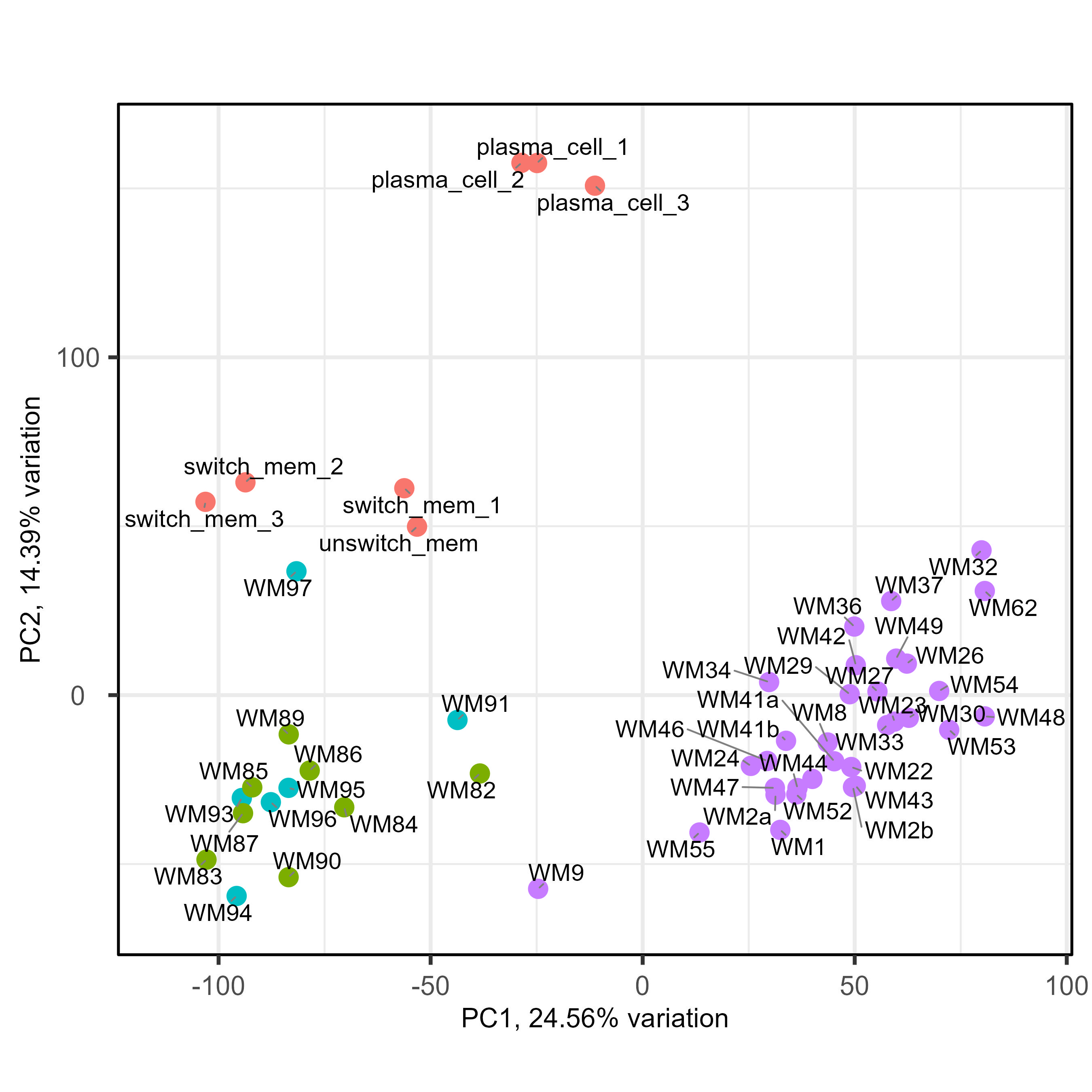
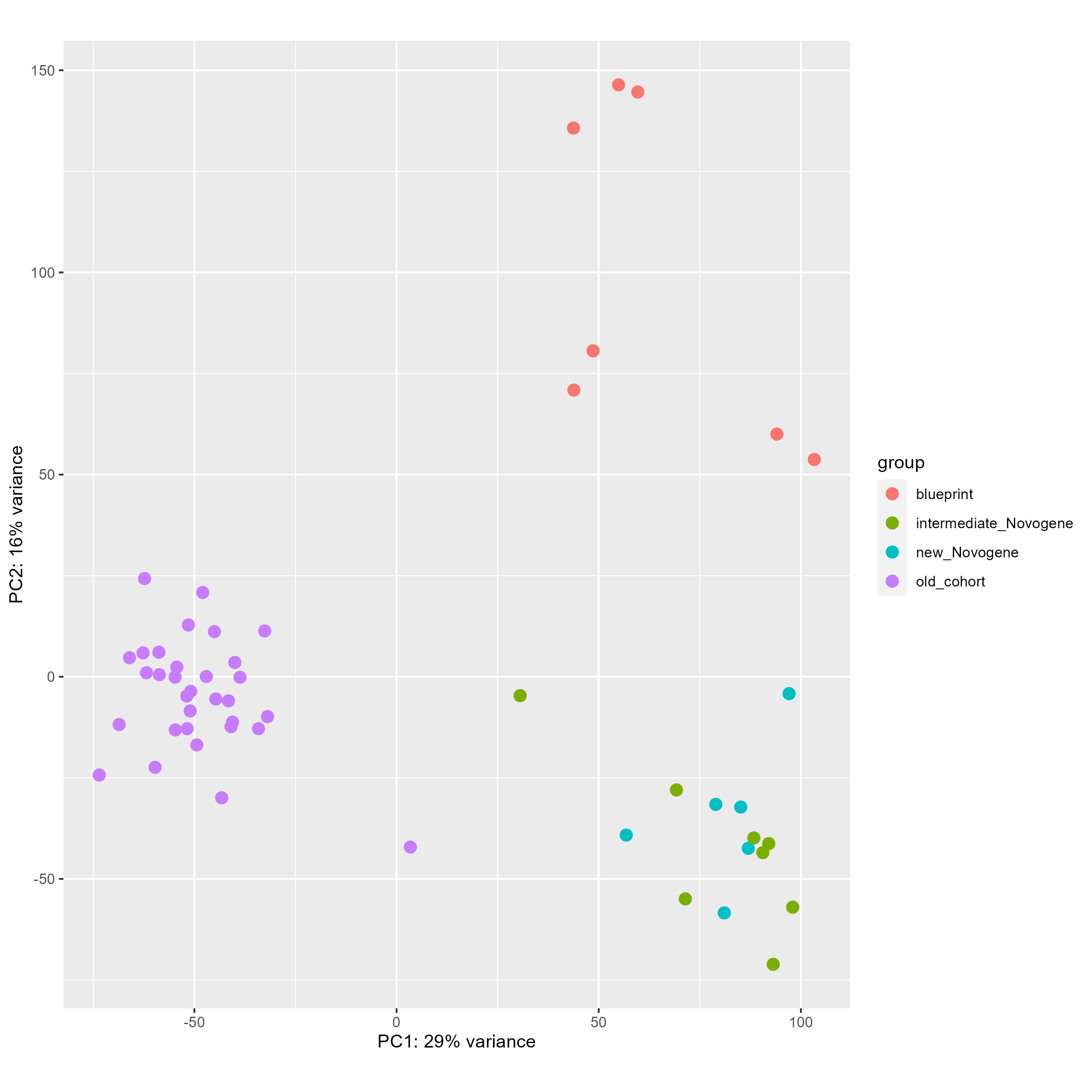
We have been fighting with a heavy batch & method effect in a cohort of bulk RNAseq from patients. As you can see below on my PCA (generated using all genes), I have three groups of samples : green and blue for patient samples done at the same place with one technology, purple for patient samples done at an other place with another technology, and red for two types of normal cells to compare patient with. As you can see the batch and method effect is very important... When doing a pairplots, I see that this batch effect can be seen the first and second PCs.
       Sample_id Disease Mutation_SPI1 Mutation_MYD Secondary_Mutation Complete_mutation                cohort cohort_for_RUVseq cohort_for_RUVseq_simpler
1            WM1      WM          SPI1          MYD               SPI1          MYD_SPI1            old_cohort        old_cohort                old_cohort
2           WM22      WM          none          MYD               none               MYD            old_cohort        old_cohort                old_cohort
3           WM23      WM          none          MYD               none               MYD            old_cohort        old_cohort                old_cohort
4           WM24      WM          none          MYD               none               MYD            old_cohort        old_cohort                old_cohort
5           WM26      WM          none          MYD              CXCR4         MYD_CXCR4            old_cohort        old_cohort                old_cohort
6           WM27      WM          none          MYD               none               MYD            old_cohort        old_cohort                old_cohort
7           WM29      WM          none          MYD       CXCR4_ARID1A  MYD_CXCR4_ARID1A            old_cohort        old_cohort                old_cohort
8           WM2a      WM          none          MYD               none               MYD            old_cohort        old_cohort                old_cohort
9           WM2b      WM          none          MYD               none               MYD            old_cohort        old_cohort                old_cohort
10          WM30      WM          none          MYD               none              none            old_cohort        old_cohort                old_cohort
11          WM31      WM          none          MYD              CXCR4         MYD_CXCR4            old_cohort        old_cohort                old_cohort
12          WM32      WM          none          MYD               none               MYD            old_cohort        old_cohort                old_cohort
13          WM33      WM          none          MYD              CXCR4         MYD_CXCR4            old_cohort        old_cohort                old_cohort
14          WM34      WM          none          MYD              CXCR4         MYD_CXCR4            old_cohort        old_cohort                old_cohort
15          WM36      WM          none          MYD               none               MYD            old_cohort        old_cohort                old_cohort
16          WM37      WM          none          MYD               none               MYD            old_cohort        old_cohort                old_cohort
17         WM41a      WM          none          MYD             ARID1A        MYD_ARID1A            old_cohort        old_cohort                old_cohort
18         WM41b      WM          none          MYD             ARID1A        MYD_ARID1A            old_cohort        old_cohort                old_cohort
19          WM42      WM          none          MYD               none               MYD            old_cohort        old_cohort                old_cohort
20          WM43      WM          none          MYD              CXCR4         MYD_CXCR4            old_cohort        old_cohort                old_cohort
21          WM44      WM          none          MYD               none              none            old_cohort        old_cohort                old_cohort
22          WM46      WM          none          MYD               none              none            old_cohort        old_cohort                old_cohort
23          WM47      WM          none          MYD               none               MYD            old_cohort        old_cohort                old_cohort
24          WM48      WM          none         none               none              none            old_cohort        old_cohort                old_cohort
25          WM49      WM          none         none               none               MYD            old_cohort        old_cohort                old_cohort
26          WM52      WM          SPI1          MYD         CXCR4_SPI1    MYD_CXCR4_SPI1            old_cohort        old_cohort                old_cohort
27          WM53      WM          none          MYD               none               MYD            old_cohort        old_cohort                old_cohort
28          WM54      WM          none          MYD               none              none            old_cohort        old_cohort                old_cohort
29          WM55      WM          none          MYD              CXCR4         MYD_CXCR4            old_cohort        old_cohort                old_cohort
30          WM62      WM          none          MYD               none               MYD            old_cohort        old_cohort                old_cohort
31           WM8      WM          none          MYD               none               MYD            old_cohort        old_cohort                old_cohort
32           WM9      WM          SPI1          MYD               SPI1          MYD_SPI1            old_cohort        old_cohort                old_cohort
33          WM91      WM       unknown      unknown            unknown           unknown          new_Novogene          Novogene                  Novogene
34          WM93      WM       unknown      unknown            unknown           unknown          new_Novogene          Novogene                  Novogene
35          WM94      WM       unknown      unknown            unknown           unknown          new_Novogene          Novogene                  Novogene
36          WM95      WM       unknown      unknown            unknown           unknown          new_Novogene          Novogene                  Novogene
37          WM96      WM       unknown      unknown            unknown           unknown          new_Novogene          Novogene                  Novogene
38          WM97      WM       unknown      unknown            unknown           unknown          new_Novogene          Novogene                  Novogene
39          WM84      WM       unknown      unknown            unknown           unknown intermediate_Novogene          Novogene                  Novogene
40          WM82      WM       unknown      unknown            unknown           unknown intermediate_Novogene          Novogene                  Novogene
41          WM86      WM       unknown      unknown            unknown           unknown intermediate_Novogene          Novogene                  Novogene
42          WM87      WM       unknown      unknown            unknown           unknown intermediate_Novogene          Novogene                  Novogene
43          WM90      WM       unknown      unknown            unknown           unknown intermediate_Novogene          Novogene                  Novogene
44          WM83      WM       unknown      unknown            unknown           unknown intermediate_Novogene          Novogene                  Novogene
45          WM89      WM       unknown      unknown            unknown           unknown intermediate_Novogene          Novogene                  Novogene
46          WM85      WM       unknown      unknown            unknown           unknown intermediate_Novogene          Novogene                  Novogene
47  switch_mem_1 Healthy    switch_mem   switch_mem         switch_mem        switch_mem             blueprint            memory                 blueprint
48  switch_mem_2 Healthy    switch_mem   switch_mem         switch_mem        switch_mem             blueprint            memory                 blueprint
49  switch_mem_3 Healthy    switch_mem   switch_mem         switch_mem        switch_mem             blueprint            memory                 blueprint
50  unswitch_mem Healthy  unswitch_mem unswitch_mem       unswitch_mem      unswitch_mem             blueprint            memory                 blueprint
51 plasma_cell_1 Healthy   plasma_cell  plasma_cell        plasma_cell       plasma_cell             blueprint       plasma_cell                 blueprint
52 plasma_cell_2 Healthy   plasma_cell  plasma_cell        plasma_cell       plasma_cell             blueprint       plasma_cell                 blueprint
53 plasma_cell_3 Healthy   plasma_cell  plasma_cell        plasma_cell       plasma_cell             blueprint       plasma_cell                 blueprint
So the idea we had was to use RUVseq, more precisely RUVg, to include correcting factor in the DESeq2 model, enabling us to correct the batch effect and compare freely samples between them. For RUVg, I tried different comparisons to determine a good dataset : purple vs only green and blue ; purple vs red vs green&blue ; purple vs green&blue vs red splitted in two (memory B cells and plasma cells). For the sake of clarity, I will only put below the code for the purple vs red vs green&blue. I tried different value of k for RUVg aswell. And then I know that I can include them like this in the DESeq2 model with "~ W1 + W2 + Complete_mutation". Here is my code :
dds <- DESeqDataSetFromTximport(txi.salmon,
                                design_file,
                                design = ~ cohort_for_RUVseq_simpler)

smallestGroupSize <- 3
keep <- rowSums(counts(dds) >= 10) >= smallestGroupSize
dds <- dds[keep,]

dds <- DESeq(dds)
vsd <- vst(dds, blind=FALSE)

res_oldcohort_novogene <- results(dds, contrast = c("cohort_for_RUVseq_simpler", "old_cohort", "Novogene"))
not_sig_oldcohort_novogene = rownames(res_oldcohort_novogene)[which(res_oldcohort_novogene$padj > 0.1)]

res_oldcohort_blueprint <- results(dds, contrast = c("cohort_for_RUVseq_simpler", "old_cohort", "blueprint"))
not_sig_oldcohort_blueprint = rownames(res_oldcohort_blueprint)[which(res_oldcohort_blueprint$padj > 0.1)]

res_Novogene_blueprint <- results(dds, contrast = c("cohort_for_RUVseq_simpler", "Novogene", "blueprint"))
not_sig_Novogene_blueprint = rownames(res_Novogene_blueprint)[which(res_Novogene_blueprint$padj > 0.1)]

not_sig_GLOBAL = Reduce(intersect,  list(not_sig_oldcohort_novogene = not_sig_oldcohort_novogene,
                                         not_sig_oldcohort_blueprint = not_sig_oldcohort_blueprint,
                                         not_sig_Novogene_blueprint = not_sig_Novogene_blueprint)) # 2653 genes

## Run RUVg sequencing

table_to_see = as.data.frame(counts(dds))

RUVg_test <- newSeqExpressionSet(counts(dds))
RUVg_test_upper_quantile_norm <- betweenLaneNormalization(RUVg_test, which="upper")

empirical <- rownames(RUVg_test_upper_quantile_norm)[ rownames(RUVg_test_upper_quantile_norm) %in% not_sig_GLOBAL ]

correction_RUVg <- RUVg(RUVg_test_upper_quantile_norm, empirical, k=2)
pdat <- pData(correction_RUVg)
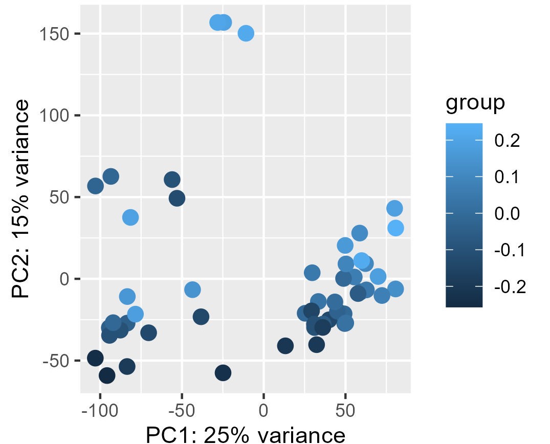
My problem is the read-out to say whether or not the correction and the factors extracted from RUVg worked properly. I have generated PCA plots colorizing the points of the PCA with the first two factors from RUVg. For the PCA (ntop = 500 and all genes), I have this for W1 from RUVg. It looks better with only the top 500 most variable genes (second picture) but this is not what I want I think...
I also extracted for the different comparisons the correlation between the W1 and W2 RUVg factors and the coordinate on PC1 and PC2 (PCA with all genes). This can be find on this table.
correlations         SIMPLER_comparison_simple
cor_W1_Dim1      0.172171
cor_W1_Dim2      0.6458019
cor_W2_Dim1      0.4765441
cor_W2_Dim2      -0.2840367
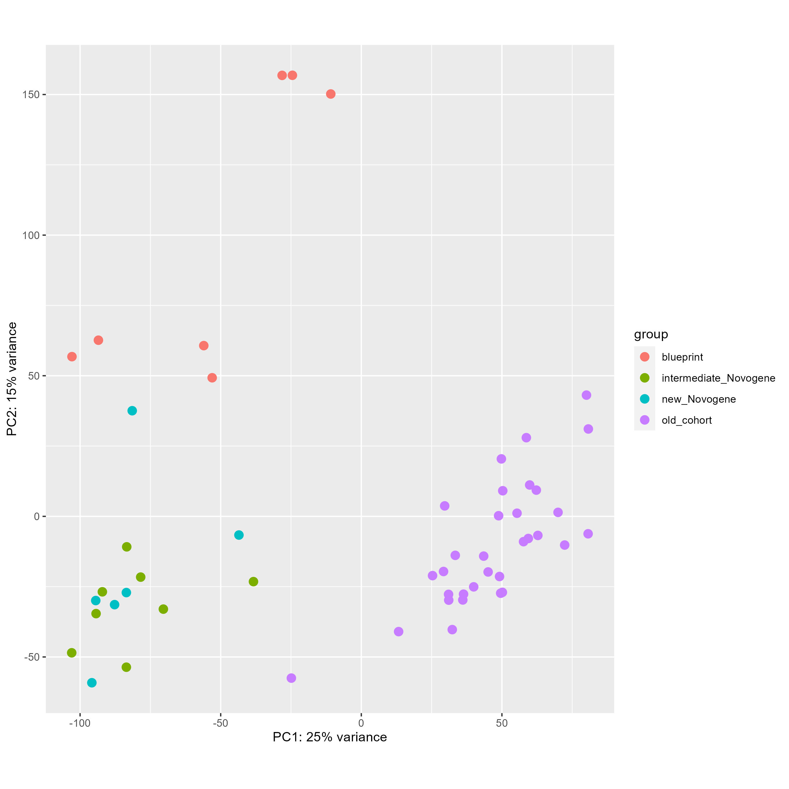
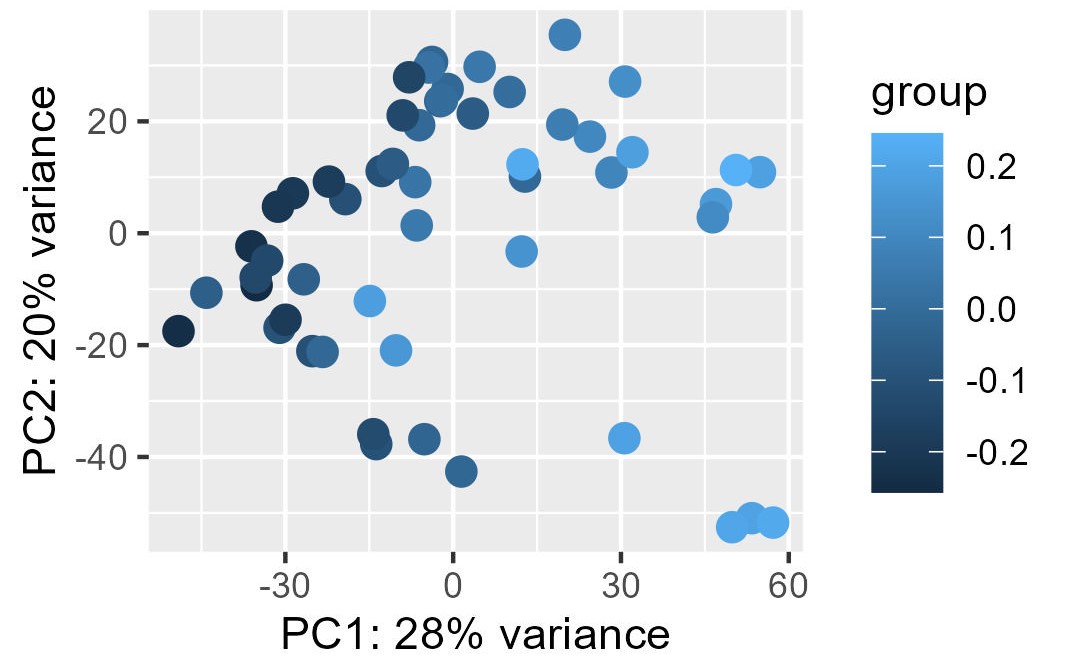
Finally, with this code here, I tried to remove this batch effect directly and see the PCA before (first picture) and after (second picture), which seems worst than without any correction.
empirical <- rownames(RUVg_test_upper_quantile_norm)[ rownames(RUVg_test_upper_quantile_norm) %in% not_sig_GLOBAL ]

correction_RUVg <- RUVg(RUVg_test_upper_quantile_norm, empirical, k=2)
pdat <- pData(correction_RUVg)

vsd <- vst(dds,blind=FALSE)
vsd_to_crush = vsd

mat <- assay(vsd)

mm <- model.matrix(~vsd$Complete_mutation, colData(vsd))

mat2 <- limma::removeBatchEffect(mat, covariates = pdat, design = mm)

assay(vsd_to_crush) = mat2

DESeq2::plotPCA(vsd, intgroup = "cohort", ntop = 100000)
DESeq2::plotPCA(vsd_to_crush, intgroup = "cohort", ntop = 100000)
My questions are the following :
1) Was I right to dive directly into RUVseq and RUVg, and did I miss something that I could do that was simpler.
2) Which read-out for the RUVg method would you use ?
3) Did I make the limma removebatcheffect function work correctly or am I missing something ?
4) If I did what needed to be done to assess the RUVg method, what would you do ? Analyse the cohort separately ?
Thank you in advance for reading and for your precious help ! Alexandre


My code for the sessionInfo() . If the pictures are too big, I will downsize them. THank you again for reading my post !