
Hi,
First a caveat: I am new to enrichment analyses, following the DESeq2 guide. The data is not mine and I have very little to say in terms of experimental design, I am just trying to improve on a "naive" analysis of producing a ration counts-per-million which exaggerates low-count reads.
I noticed something counter-intuitive in my data, namely that lfcShrink does the opposite of what it should: low-count reads are exaggerated and high-count reads are shrunk.
Two example genes below.
# counts, metadata defined elsewhere
> dds <- DESeq2::DESeqDataSetFromMatrix(
    countData = counts,
    colData = metadata,
    design = ~condition
  )
> dds$condition <- relevel(dds$condition, ref = "reference")

# many zeros in this dataset hence poscount
> dds <- DESeq2::DESeq(dds, sfType = "poscount")

> result_unshrunk <- results(dds, name = "condition_condition1_vs_reference")
> result_unshrunk[c('gene1', 'gene2'),]

log2 fold change (MLE): condition1 vs reference
Wald test p-value: condition1 vs reference
DataFrame with 2 rows and 6 columns
       baseMean log2FoldChange     lfcSE      stat     pvalue      padj
      <numeric>      <numeric> <numeric> <numeric>  <numeric> <numeric>
gene1   11.0575       -5.49035   2.08908  -2.62811 0.00858602  0.116205
gene2 7537.5202        8.97127   5.23205   1.71468 0.08640462  0.289067

> result_apeglm <- lfcShrink(dds, coef = "condition_condition1_vs_reference", type = "apeglm")
> result_apeglm[c('gene1', 'gene2'),]

log2 fold change (MAP): condition1 vs reference
Wald test p-value: condition1 vs reference
DataFrame with 2 rows and 5 columns
       baseMean log2FoldChange     lfcSE     pvalue      padj
      <numeric>      <numeric> <numeric>  <numeric> <numeric>
gene1   11.0575      10.457654        NA 0.00858602  0.116205
gene2 7537.5202       0.123898        NA 0.08640462  0.289067
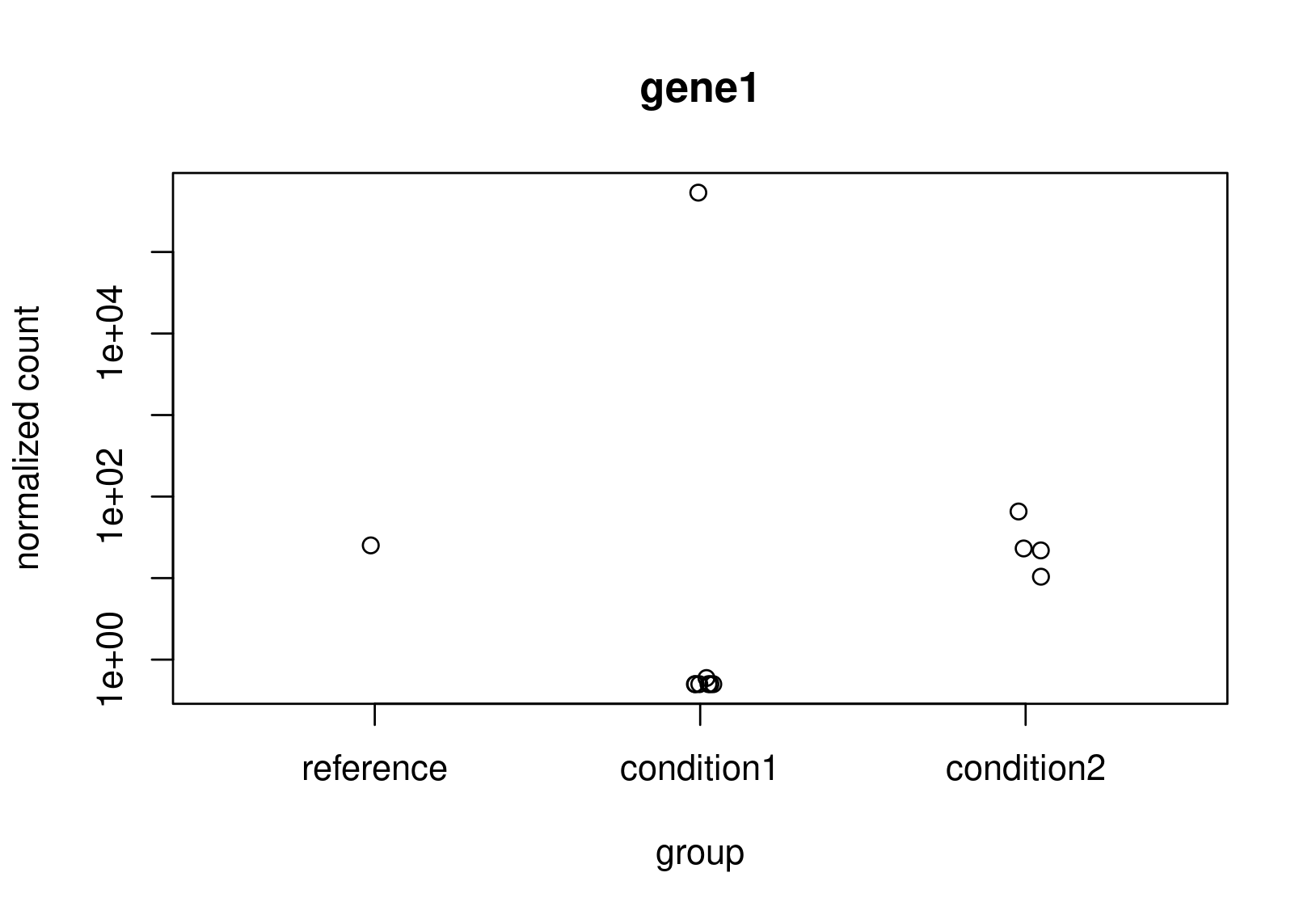
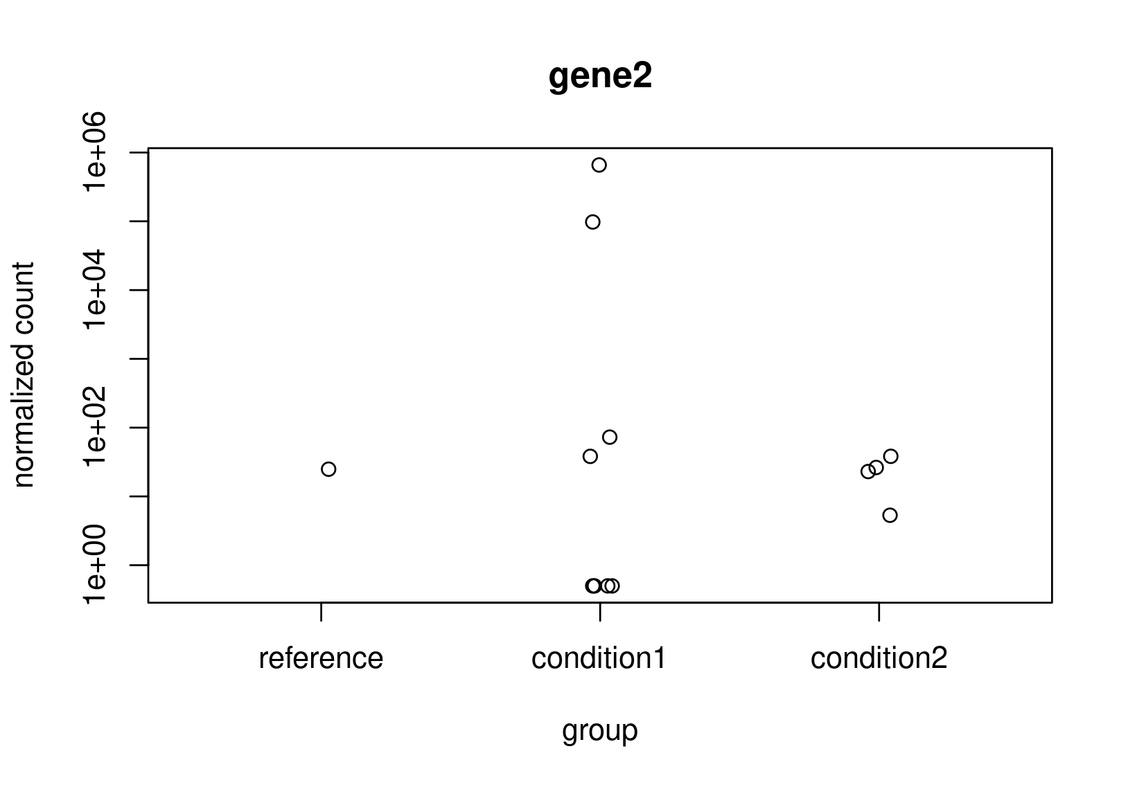
Looking at the normalized counts below (from plotCounts). It seems obvious to me that gene2 should be the one with higher LFC. Both genes have the same counts in reference, but one has a clearly higher average. In the un-shrunk calculation gene2 is higher, but the relationship reverses under the shrunk model.
Now, this is just a small snapshot of the data, which I cannot share, so I appreciate that it's not possible to some up with a definitive answer via a forum. Still, I would appreciate some guidance as to how to diagnose what is really happening?
Below are the distributions from plotMA.
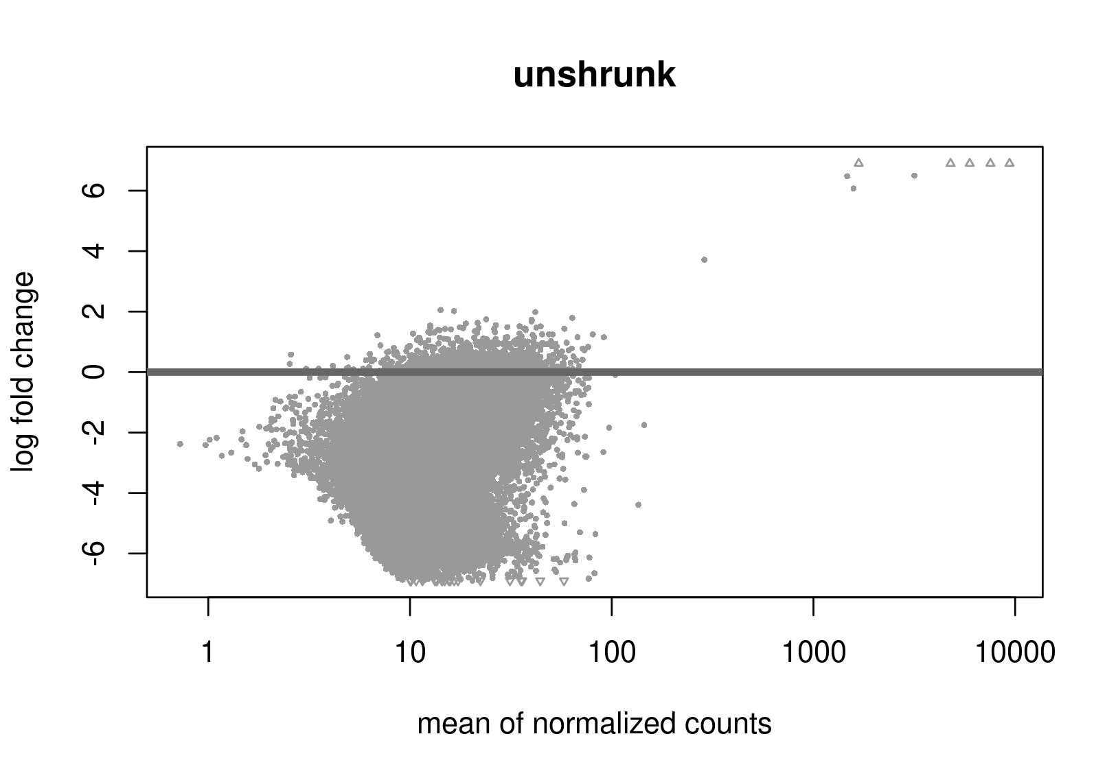
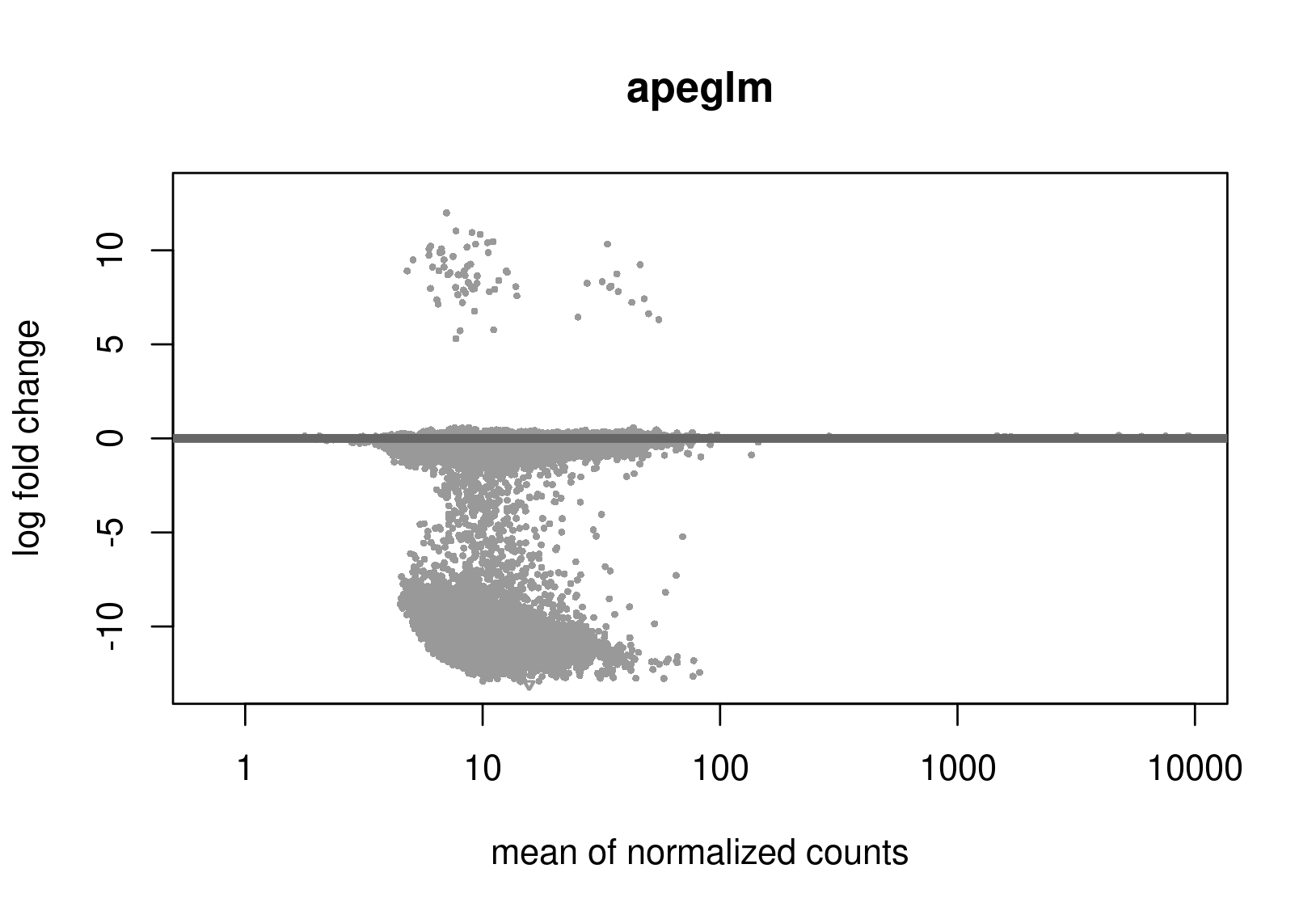
Does this give a hint? Perhaps it's the non-symmetric LFC distribution that's the problem? Thanks a lot for any help.


Is this RNA-seq? The unshrunken MA-plot looks very odd and indicates that normalization is completely offset.
I agree it looks offset (and weird). The data is from NGS, not RNAseq, but we still want to see relative abundance between conditions - I thought the same principles would apply.