Entering edit mode

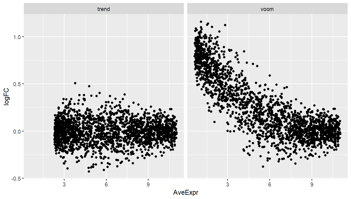
I am running both limma-voom and limma-trend on simulated data of two experimental groups where the only main difference is that group-A has double library size compared to group-B. While limma-trend produces an expected MA-plot (below), voom seems to fail here, and I wonder why.
I know that the data are mocked up, but I encountered a more extreme plot on a real dataset where library size was nested by group, and voom produced MA-plots that was not only skewed as this one here, but also the bulk of datapoints was well offset from y=0 (seemingly not correcting properly for library size). Any pointers?
suppressMessages(library(scuttle))

set.seed(1)
sce <- mockSCE(ncells = 1000, ngenes = 2000)
sce$condition <- factor(rep(LETTERS[1:2], each=500))
# double library size for "A" group
assay(sce)[,1:500] <- assay(sce)[,1:500]*2

library(scran)
y <- convertTo(sce, type="edgeR")

library(limma)
#>
#> Attaching package: 'limma'
#> The following object is masked from 'package:BiocGenerics':
#>
#>     plotMA
library(edgeR)
#>
#> Attaching package: 'edgeR'
#> The following object is masked from 'package:SingleCellExperiment':
#>
#>     cpm
design <- model.matrix(~condition, y$samples)

v_voom <- eBayes(voomLmFit(y, design))
v_trend <- eBayes(lmFit(edgeR::cpm(y, log=TRUE), design), trend = TRUE)

res_voom <- topTable(v_voom, coef=2, number = Inf)
res_voom$x <- "voom"

res_trend <- topTable(v_trend, coef=2, number = Inf)
res_trend$x <- "trend"

res <- rbind(res_voom, res_trend)

library(ggplot2)
ggplot(res, aes(x=AveExpr, y=logFC)) +
  geom_point() +
  facet_wrap(~x)


sessionInfo()
#> R version 4.4.1 (2024-06-14 ucrt)
#> Platform: x86_64-w64-mingw32/x64
#> Running under: Windows 11 x64 (build 22000)
#>
#> Matrix products: default
#>
#>
#> locale:
#> [1] LC_COLLATE=English_Germany.utf8  LC_CTYPE=English_Germany.utf8
#> [3] LC_MONETARY=English_Germany.utf8 LC_NUMERIC=C
#> [5] LC_TIME=English_Germany.utf8
#>
#> time zone: Europe/London
#> tzcode source: internal
#>
#> attached base packages:
#> [1] stats4    stats     graphics  grDevices utils     datasets  methods
#> [8] base
#>
#> other attached packages:
#>  [1] ggplot2_3.5.1               edgeR_4.2.1
#>  [3] limma_3.60.4                scran_1.32.0
#>  [5] scuttle_1.14.0              SingleCellExperiment_1.26.0
#>  [7] SummarizedExperiment_1.34.0 Biobase_2.64.0
#>  [9] GenomicRanges_1.56.1        GenomeInfoDb_1.40.1
#> [11] IRanges_2.38.1              S4Vectors_0.42.1
#> [13] BiocGenerics_0.50.0         MatrixGenerics_1.16.0
#> [15] matrixStats_1.3.0
#>
#> loaded via a namespace (and not attached):
#>  [1] gtable_0.3.5              xfun_0.47
#>  [3] lattice_0.22-6            generics_0.1.3
#>  [5] vctrs_0.6.5               tools_4.4.1
#>  [7] parallel_4.4.1            fansi_1.0.6
#>  [9] tibble_3.2.1              cluster_2.1.6
#> [11] pkgconfig_2.0.3           BiocNeighbors_1.22.0
#> [13] Matrix_1.7-0              sparseMatrixStats_1.16.0
#> [15] dqrng_0.4.1               lifecycle_1.0.4
#> [17] GenomeInfoDbData_1.2.12   farver_2.1.2
#> [19] compiler_4.4.1            munsell_0.5.1
#> [21] statmod_1.5.0             bluster_1.14.0
#> [23] codetools_0.2-20          htmltools_0.5.8.1
#> [25] yaml_2.3.10               pillar_1.9.0
#> [27] crayon_1.5.3              BiocParallel_1.38.0
#> [29] DelayedArray_0.30.1       abind_1.4-5
#> [31] tidyselect_1.2.1          rsvd_1.0.5
#> [33] locfit_1.5-9.10           metapod_1.12.0
#> [35] digest_0.6.37             dplyr_1.1.4
#> [37] BiocSingular_1.20.0       labeling_0.4.3
#> [39] splines_4.4.1             fastmap_1.2.0
#> [41] grid_4.4.1                colorspace_2.1-1
#> [43] cli_3.6.3                 SparseArray_1.4.8
#> [45] magrittr_2.0.3            S4Arrays_1.4.1
#> [47] utf8_1.2.4                withr_3.0.1
#> [49] scales_1.3.0              DelayedMatrixStats_1.26.0
#> [51] UCSC.utils_1.0.0          rmarkdown_2.28
#> [53] XVector_0.44.0            httr_1.4.7
#> [55] igraph_2.0.3              ScaledMatrix_1.12.0
#> [57] beachmat_2.20.0           evaluate_0.24.0
#> [59] knitr_1.48                irlba_2.3.5.1
#> [61] rlang_1.1.4               Rcpp_1.0.13
#> [63] glue_1.7.0                reprex_2.1.1
#> [65] rstudioapi_0.16.0         jsonlite_1.8.8
#> [67] R6_2.5.1                  fs_1.6.4
#> [69] zlibbioc_1.50.0
Created on 2024-08-26 with reprex v2.1.1

I would recommend reading RNA-seq analysis is easy as 1-2-3 with limma, Glimma and edgeR first.
After creating the
DGEList,y, if you viewy$samples, you will see that all the values in thenorm.factorscolumn are 1. The library sizes are being treated as equal, by default. You first need to remove low-count features and calculate library size scaling factors, like so:If you check
y$samples$norm.factors, they are now updated.However, this does not seem to result in a "correct" looking plot:
I think this just has to do with how the data was simulated, since the plot that results from the following is not something you would ever see with real data (see Figure 4 in the paper linked above for an example):
I know all these workflows, and it does not apply. Normalization factors correct for composition, not depth. The issue is depth here. With all NFs being 1 the library size is simply multiplied by one to form the effective library size. I think you misinterpret what normalization factors do in limma.
As said, it's a dummy example for a real dataset I cannot easily share here. It's single-cell data (not pseudobulk) so the standard prefilters and normalization does not apply. The point stands as why trend and voom are different here, given that their inference is typically very similar. In the real data prefiltering via percent of expression per cluster is done, and normalization, whether done by just library size or deconvolution factors from scran, have no notable effect -- the MA-plot is well offset, which is not the case when using trend, but voom.