Large logFC but somewhat high FDR
1
0
Entering edit mode
JKim • 0
@4035f8c1
Last seen 9 minutes ago
United States

Hi Limpa developers,

Thank you for the great package! I'm so happy to use it.

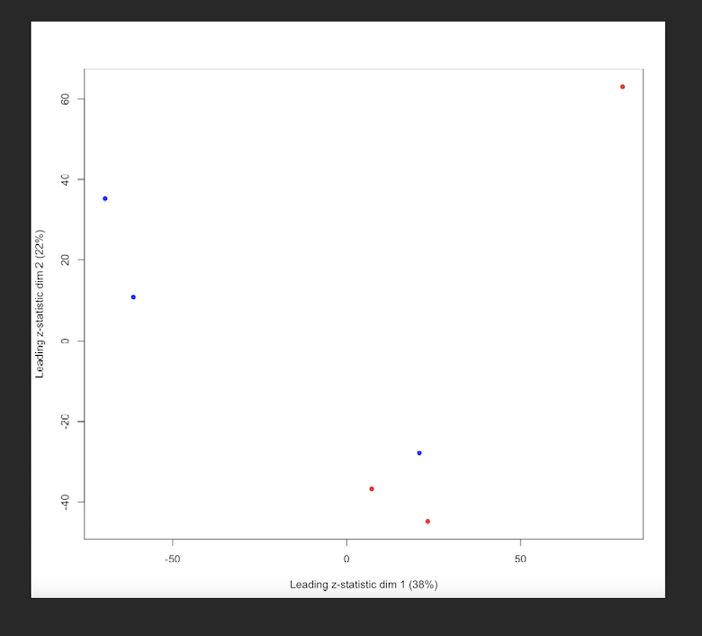
I have a protein level intensity table (around 4600 proteins inferred) from a mouse experiment (3 WT samples and 3 KO samples, WT is the reference level). After running limpa, I noticed that some proteins show large logFC but still have relatively high FDR, which is confusing to me. The MDS plot suggests that there are outlier samples, so my gut feeling is that these samples increased within group variability, leading to high pvalues and FDRs. Having only 3 replicates doesn't much help either.

I followed limpa's vignettes but used fit2 <- eBayes(fit2, robust=T) and limma::normalizeBetweenArrays(method = "cyclicloess").


> topTable(fit2, coef="KO_vs_WT", confint = T) |> head()
                                           PROTEIN GENE_SYMBOL ACCESSION NPeptides   PropObs     logFC       CI.L      CI.R   AveExpr         t
O55226                              Chondroadherin        Chad    O55226         1 1.0000000  2.238540  1.4998398  2.977240  7.056010  6.710509
P15501          Prostatic spermine-binding protein         Sbp    P15501         1 0.8333333 -5.597560 -7.5481291 -3.646991  8.536706 -6.469931
Q9DCM0 Persulfide dioxygenase ETHE1, mitochondrial       Ethe1    Q9DCM0         1 1.0000000  1.608751  0.9927308  2.224770 10.408467  5.782997
Q9EPW4      C-type lectin domain family 3 member A      Clec3a    Q9EPW4         1 0.8333333  2.820516  1.8020354  3.838997  5.828143  6.132459
Q91YN1                             Protein FAM118A     Fam118a    Q91YN1         1 1.0000000  1.680796  1.0213627  2.340229  7.242839  5.644208
P60840                           Alpha-endosulfine        Ensa    P60840         1 1.0000000 -2.040405 -2.8418892 -1.238921  6.902121 -5.637418
             P.Value adj.P.Val         B
O55226 0.00004221111 0.1205903 1.9886820
P15501 0.00010441290 0.1205903 1.2256714
Q9DCM0 0.00014770557 0.1205903 1.1486875
Q9EPW4 0.00009090405 0.1205903 1.1429693
Q91YN1 0.00017995052 0.1205903 0.9074773
P60840 0.00018170999 0.1205903 0.8761251

For example, when I looked at the P15501 and O55226 normalized log2 intensities from y.protein$E, they seem differentially expressed to my eye (sorry about the poor wording), yet somewhat high FDR, which I find it baffling...

| ACCESSION | GENE_SYMBOL | WT1    | WT2   | WT3    | KO1   | KO2   | KO3   |
| --------- | ----------- | ------ | ----- | ------ | ----- | ----- | ----- |
| O55226    | Chad        | 5.917  | 6.013 | 5.879  | 8.666 | 7.773 | 8.087 |
| P15501    | Sbp         | 11.959 | 9.416 | 11.920 | 7.834 | 4.325 | 5.767 |

MDS plot - Red represents WT and blue represents KO.
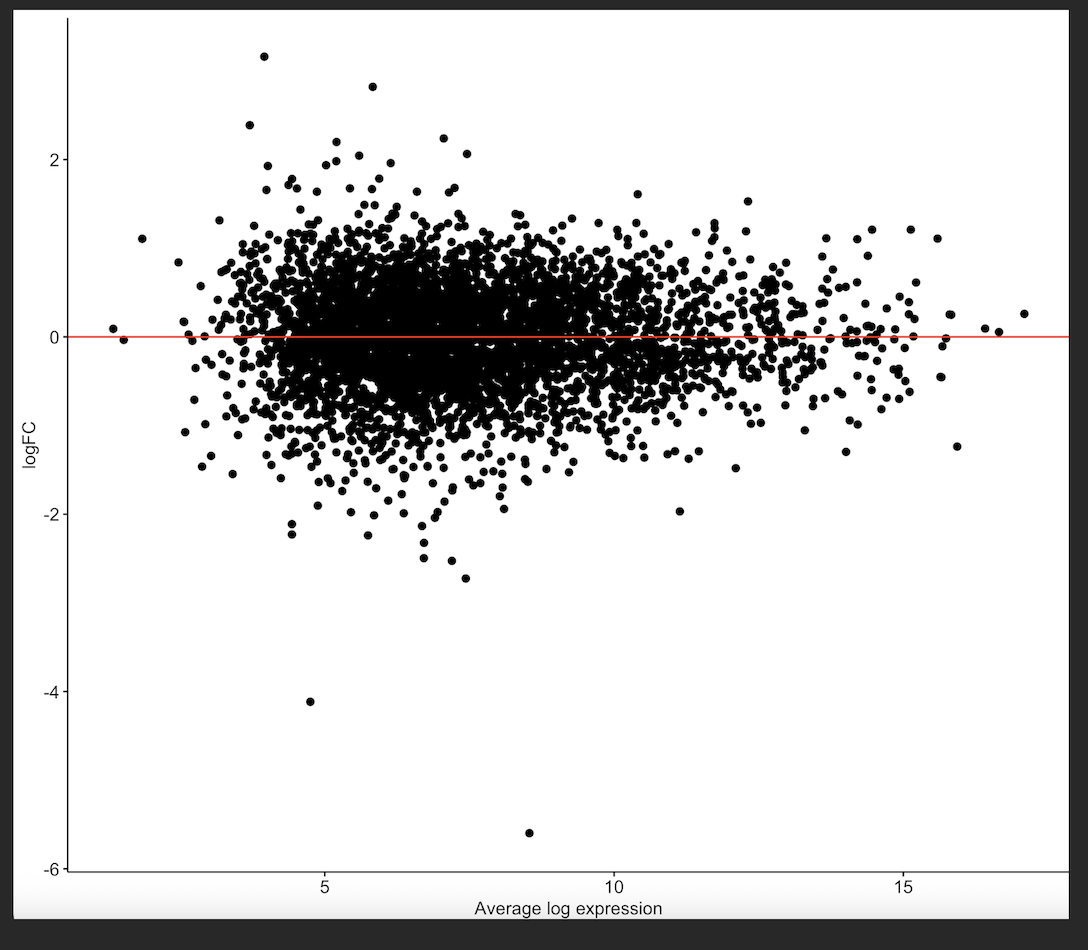
enter image description here

MD plot

enter image description here

limpa • 104 views
ADD COMMENT
0
Entering edit mode

forgot to attach some other plots, which may be informative...

RLE plot, after normalization

enter image description here

pvalue distribution

enter image description here

Well, I got duplicate FDRs. For those wondering why there are duplicate adjusted p-values, see p.adjust BH generates duplicate values

ADD REPLY
0
Entering edit mode

I don't know what tp1 is. The relevant histogram would be:

hist(fit2$p.value[,"KO_vs_WT"])
ADD REPLY
1
Entering edit mode
@gordon-smyth
Last seen 11 hours ago
WEHI, Melbourne, Australia

Glad you're getting good use out of the package.

The results that you show seem pretty much as one would expect, with nothing surprising. The MDS plot shows huge intra-group variability, with no clear separation between WT and KO, so one would not expect to get significant proteins. One of the WT samples clusters with two of the KO samples.

The two proteins that you show (Chad and Sbp), do look DE if analysed by themselves, and limpa is giving you very small p-values for them (P = 0.000042), so limpa is agreeing with you. Indeed, limpa is giving smaller p-values that you would get from doing ordinary t-tests on these proteins.

However, you didn't select Chat and Sbp in advance, so you have to adjust for multiple testing. The Bonferroni adjusted p-value for Chad would be 4600 * 0.000042 = 0.194 so, again, limpa is doing a bit better than a naive adjustment.

What can you do?

  • Investigate why there's so much between-sample variability. Anything unusual about the two outlier samples?

  • Use sample.weights=TRUE when you run dpcDE(), to downweight the two outlier samples. That will give lower p-values.

  • Use a FDR cutoff of 0.2 instead of 0.05. There's no scientific rule that says you need to use FDR < 0.05. A FDR cutoff of 0.2 still means that over 80% of the putative DE proteins are correct.

  • Use propTrueNULL(fit2$p.value[,"KO_vs_WT"]) to estimate the proportion of truly DE proteins.

ADD COMMENT
0
Entering edit mode

Thank you very much for taking the time to answer the question. I really appreciate your insights and comments.

ADD REPLY

Login before adding your answer.

Traffic: 855 users visited in the last hour
Help About
FAQ
Access RSS
API
Stats

Use of this site constitutes acceptance of our User Agreement and Privacy Policy.

Powered by the version 2.3.6