
Hi,
I have a microRNA dataset, and I have samples from 2 suborders, 5 families, and 7 species.
I would like to find differentially expressed microRNAs to then conduct functional enrichment with like gene ontology, or KEGG pathway.
I first checked the data for patterns using PCA and clustering, and I first used the normalized counts
norm_cetaceans <- counts(res_27_cets, normalized = TRUE)
But later I found that it is suggested to use either VST or rlog transformation so I used VST for the exploratory analysis.
Are exploratory analysis with VST equivalent with the normalized counts from DESeq()?
Also, I checked the VST dataset, and some values are negative, is this okay, expected?
head(counts_VST_19, c(6L, 6L))
| 135208-DM-Ttru 135209-ET-Ttru 137808-DM-Ttru 137809-ET-Ttru 145459-Ddel 145462-Ddel |
|---|
| hsa-miR-324-3p -3.658031 4.448456 -3.658031 -3.658031 2.9010645 -3.658031 |
| hsa-miR-212-3p -3.658031 -3.658031 -3.658031 -3.658031 -3.6580309 -3.658031 |
| hsa-miR-660-5p 7.108520 6.469499 7.325406 7.607373 8.0828895 7.469345 |
| hsa-miR-670-3p -3.658031 -3.658031 -3.658031 -3.658031 -3.6580309 -3.658031 |
| hsa-miR-876-3p -3.658031 -3.658031 -3.658031 -3.658031 -3.6580309 -3.658031 |
| hsa-miR-382-3p -3.658031 -3.658031 -3.658031 -3.658031 -0.7916052 -3.658031 |
Also, in the exploratory analysis section, it uses the code:
vsd <- vst(dds, blind = FALSE)
Shouldn't one use blind=T?
In the website it says : "In the above function calls, we specified blind = FALSE, which means that differences between cell lines and treatment (the variables in the design) will not contribute to the expected variance-mean trend of the experiment", while on the R ?help states: blind logical, whether to blind the transformation to the experimental design. blind=TRUE should be used for comparing samples in a manner unbiased by prior information on samples, for example to perform sample QA (quality assurance).
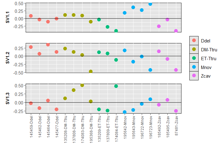
In the RNA-seq workflow it mentions using svaseq to identify Removing hidden batch effects. After the exploratory analysis, some samples showed ill-behavior, not clustering with its species, far away in the dendrogram/PCA (3D). After removing those, I did PCA and clustering, and the dataset looked better. I am undecided whether it is beneficial or recommended to check for hidden batch effects. For instance, after removing the weird samples, many microRNAs were removed due to all-zeros.
Here are the plots for SVA - using 3 surrogate variables suggested by .
I also wanted to mention that I have 4 species, but I also want to analyse and find DE-microRNAs at the family (3 groups) and suborder level (2). When I add the design ~ Suborder + Family, DESEq mentions that the groups are linear combinations of others. Is this error normal, so that I have to use separate designs?
Finally, as I said, I want to get the DE-mircroRNAs, and do an enrichment analysis but I am confused about how to proceed. I read that one should use the padjust values and rank the microRNAs (genes) by lfcShrink, but my confusing is that lfcShrink also adjusts padjust values. It seems weird that I used the padjust values from results but then use the log2FoldChange from lfcShrink - which is a different "matrix" with different padjust values.
Sorry for the questions, I want to make sure that I am proceeding the right way.
Thanks
sessionInfo( )
R version 4.3.2 (2023-10-31 ucrt) Platform: x86_64-w64-mingw32/x64 (64-bit) Running under: Windows 11 x64 (build 26100)
Matrix products: default
locale:
1 LC_COLLATE=English_United States.utf8 LC_CTYPE=English_United States.utf8
[3] LC_MONETARY=English_United States.utf8 LC_NUMERIC=C
[5] LC_TIME=English_United States.utf8
time zone: America/New_York tzcode source: internal
attached base packages: 1 stats4 stats graphics grDevices utils datasets methods base
other attached packages:
1 sva_3.50.0 BiocParallel_1.36.0 mgcv_1.9-3
[4] nlme_3.1-168 SWATH2stats_1.32.1 IHW_1.30.0
[7] genefilter_1.84.0 ggdendro_0.2.0 gridExtra_2.3
[10] tsne_0.1-3.1 glmpca_0.2.0 RColorBrewer_1.1-3
[13] PoiClaClu_1.0.2.1 umap_0.2.10.0 plotly_4.11.0
[16] lubridate_1.9.4 forcats_1.0.1 stringr_1.6.0
[19] dplyr_1.1.4 purrr_1.0.4 readr_2.1.6
[22] tidyr_1.3.1 tibble_3.2.1 tidyverse_2.0.0
[25] factoextra_1.0.7 FactoMineR_2.12 pheatmap_1.0.13
[28] gplots_3.2.0 scales_1.4.0 ggpubr_0.6.2
[31] ggplot2_4.0.0 DESeq2_1.42.1 SummarizedExperiment_1.32.0
[34] Biobase_2.62.0 MatrixGenerics_1.14.0 matrixStats_1.5.0
[37] GenomicRanges_1.54.1 GenomeInfoDb_1.38.8 IRanges_2.36.0
[40] S4Vectors_0.40.2 BiocGenerics_0.48.1
loaded via a namespace (and not attached):
1 splines_4.3.2 later_1.4.4 filelock_1.0.3 bitops_1.0-9
[5] lpsymphony_1.30.0 XML_3.99-0.20 lifecycle_1.0.4 rstatix_0.7.3
[9] edgeR_4.0.16 processx_3.8.6 lattice_0.22-7 MASS_7.3-60
[13] flashClust_1.01-2 crosstalk_1.2.2 backports_1.5.0 magrittr_2.0.4
[17] limma_3.58.1 yaml_2.3.10 remotes_2.5.0 httpuv_1.6.16
[21] otel_0.2.0 askpass_1.2.1 sessioninfo_1.2.3 pkgbuild_1.4.8
[25] reticulate_1.44.1 DBI_1.2.3 cowplot_1.2.0 multcomp_1.4-29
[29] abind_1.4-8 pkgload_1.4.1 zlibbioc_1.48.2 RCurl_1.98-1.17
[33] TH.data_1.1-5 rappdirs_0.3.3 sandwich_3.1-1 GenomeInfoDbData_1.2.11
[37] ggrepel_0.9.6 RSpectra_0.16-2 annotate_1.80.0 codetools_0.2-20
[41] DelayedArray_0.28.0 xml2_1.5.1 DT_0.34.0 tidyselect_1.2.1
[45] farver_2.1.2 BiocFileCache_2.10.2 jsonlite_2.0.0 ellipsis_0.3.2
[49] Formula_1.2-5 survival_3.8-3 emmeans_2.0.1 bbmle_1.0.25.1
[53] progress_1.2.3 tools_4.3.2 Rcpp_1.1.0 glue_1.8.0
[57] SparseArray_1.2.4 usethis_3.2.1 withr_3.0.2 numDeriv_2016.8-1.1
[61] BiocManager_1.30.27 fastmap_1.2.0 openssl_2.3.4 callr_3.7.6
[65] caTools_1.18.3 digest_0.6.37 timechange_0.3.0 R6_2.6.1
[69] mime_0.13 estimability_1.5.1 colorspace_2.1-2 gtools_3.9.5
[73] biomaRt_2.58.2 RSQLite_2.4.5 dichromat_2.0-0.1 utf8_1.2.6
[77] generics_0.1.4 ggsci_4.2.0 data.table_1.17.8 prettyunits_1.2.0
[81] httr_1.4.7 htmlwidgets_1.6.4 S4Arrays_1.2.1 scatterplot3d_0.3-44
[85] pkgconfig_2.0.3 gtable_0.3.6 blob_1.2.4 S7_0.2.0
[89] XVector_0.42.0 htmltools_0.5.8.1 carData_3.0-5 profvis_0.4.0
[93] multcompView_0.1-10 leaps_3.2 png_0.1-8 rstudioapi_0.17.1
[97] reshape2_1.4.5 tzdb_0.5.0 coda_0.19-4.1 curl_7.0.0
[101] bdsmatrix_1.3-7 zoo_1.8-14 cachem_1.1.0 KernSmooth_2.23-26
[105] parallel_4.3.2 miniUI_0.1.2 AnnotationDbi_1.64.1 desc_1.4.3
[109] apeglm_1.24.0 pillar_1.11.1 grid_4.3.2 vctrs_0.6.5
[113] slam_0.1-55 urlchecker_1.0.1 promises_1.5.0 car_3.1-3
[117] dbplyr_2.5.1 xtable_1.8-4 cluster_2.1.8.1 mvtnorm_1.3-3
[121] cli_3.6.4 locfit_1.5-9.12 compiler_4.3.2 rlang_1.1.5
[125] crayon_1.5.3 ggsignif_0.6.4 fdrtool_1.2.18 labeling_0.4.3
[129] emdbook_1.3.14 ps_1.9.1 plyr_1.8.9 fs_1.6.6
[133] stringi_1.8.7 viridisLite_0.4.2 Biostrings_2.70.3 lazyeval_0.2.2
[137] devtools_2.4.5 Matrix_1.6-4 hms_1.1.4 bit64_4.6.0-1
[141] statmod_1.5.1 KEGGREST_1.42.0 shiny_1.12.1 broom_1.0.11
[145] memoise_2.0.1 bit_4.6.0
```


Hi ATpoint Thanks for the information. Could you please expand on when to use adjusted p-values vs nominal p-values. My understanding was that due to multiple testing, corrected p-values were supposed to be used, and that one should use those genes/microRNAs that passed the significance threshold for downstream analysis like functional enrichment. Statistical significance is one aspect - to avoid spurious results, but the other important aspect is effect size, in my case biological impact/difference. For instance, one microRNA had a p-adjust of 0.00009 but the LFC was 0.1, the expression difference was statistically significant but the effect size was very small. Thus, my idea was to retain and analyze only the microRNAs with p-adjust < 0.1 and LFC higher than 0.5 or lower than -0.5. I would appreciate a lot if you could explain why should p-values be used with LFC instead of adjusted p-values. Thanks