
Hi,
I have a microRNA dataset, and I have samples from 2 suborders, 5 families, and 7 species.
I would like to find differentially expressed microRNAs to then conduct functional enrichment with like gene ontology, or KEGG pathway.
I first checked the data for patterns using PCA and clustering, and I first used the normalized counts
norm_cetaceans <- counts(res_27_cets, normalized = TRUE)
But later I found that it is suggested to use either VST or rlog transformation so I used VST for the exploratory analysis.
Are exploratory analysis with VST equivalent with the normalized counts from DESeq()?
Also, I checked the VST dataset, and some values are negative, is this okay, expected?
head(counts_VST_19, c(6L, 6L))
| 135208-DM-Ttru 135209-ET-Ttru 137808-DM-Ttru 137809-ET-Ttru 145459-Ddel 145462-Ddel |
|---|
| hsa-miR-324-3p -3.658031 4.448456 -3.658031 -3.658031 2.9010645 -3.658031 |
| hsa-miR-212-3p -3.658031 -3.658031 -3.658031 -3.658031 -3.6580309 -3.658031 |
| hsa-miR-660-5p 7.108520 6.469499 7.325406 7.607373 8.0828895 7.469345 |
| hsa-miR-670-3p -3.658031 -3.658031 -3.658031 -3.658031 -3.6580309 -3.658031 |
| hsa-miR-876-3p -3.658031 -3.658031 -3.658031 -3.658031 -3.6580309 -3.658031 |
| hsa-miR-382-3p -3.658031 -3.658031 -3.658031 -3.658031 -0.7916052 -3.658031 |
Also, in the exploratory analysis section, it uses the code:
vsd <- vst(dds, blind = FALSE)
Shouldn't one use blind=T?
In the website it says : "In the above function calls, we specified blind = FALSE, which means that differences between cell lines and treatment (the variables in the design) will not contribute to the expected variance-mean trend of the experiment", while on the R ?help states: blind logical, whether to blind the transformation to the experimental design. blind=TRUE should be used for comparing samples in a manner unbiased by prior information on samples, for example to perform sample QA (quality assurance).
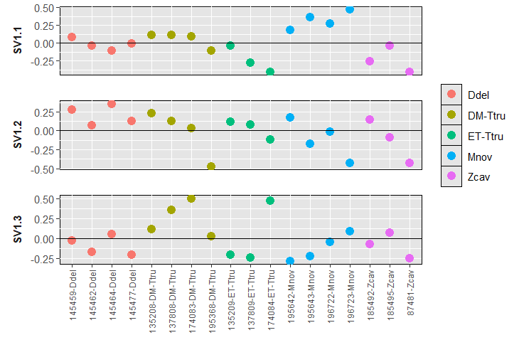
In the RNA-seq workflow it mentions using svaseq to identify Removing hidden batch effects. After the exploratory analysis, some samples showed ill-behavior, not clustering with its species, far away in the dendrogram/PCA (3D). After removing those, I did PCA and clustering, and the dataset looked better. I am undecided whether it is beneficial or recommended to check for hidden batch effects. For instance, after removing the weird samples, many microRNAs were removed due to all-zeros.
Here are the plots for SVA - using 3 surrogate variables suggested by .
I also wanted to mention that I have 4 species, but I also want to analyse and find DE-microRNAs at the family (3 groups) and suborder level (2). When I add the design ~ Suborder + Family, DESEq mentions that the groups are linear combinations of others. Is this error normal, so that I have to use separate designs?
Finally, as I said, I want to get the DE-mircroRNAs, and do an enrichment analysis but I am confused about how to proceed. I read that one should use the padjust values and rank the microRNAs (genes) by lfcShrink, but my confusing is that lfcShrink also adjusts padjust values. It seems weird that I used the padjust values from results but then use the log2FoldChange from lfcShrink - which is a different "matrix" with different padjust values.
Sorry for the questions, I want to make sure that I am proceeding the right way.
Thanks
sessionInfo( )
R version 4.3.2 (2023-10-31 ucrt) Platform: x86_64-w64-mingw32/x64 (64-bit) Running under: Windows 11 x64 (build 26100)
Matrix products: default
locale:
1 LC_COLLATE=English_United States.utf8 LC_CTYPE=English_United States.utf8
[3] LC_MONETARY=English_United States.utf8 LC_NUMERIC=C
[5] LC_TIME=English_United States.utf8
time zone: America/New_York tzcode source: internal
attached base packages: 1 stats4 stats graphics grDevices utils datasets methods base
other attached packages:
1 sva_3.50.0 BiocParallel_1.36.0 mgcv_1.9-3
[4] nlme_3.1-168 SWATH2stats_1.32.1 IHW_1.30.0
[7] genefilter_1.84.0 ggdendro_0.2.0 gridExtra_2.3
[10] tsne_0.1-3.1 glmpca_0.2.0 RColorBrewer_1.1-3
[13] PoiClaClu_1.0.2.1 umap_0.2.10.0 plotly_4.11.0
[16] lubridate_1.9.4 forcats_1.0.1 stringr_1.6.0
[19] dplyr_1.1.4 purrr_1.0.4 readr_2.1.6
[22] tidyr_1.3.1 tibble_3.2.1 tidyverse_2.0.0
[25] factoextra_1.0.7 FactoMineR_2.12 pheatmap_1.0.13
[28] gplots_3.2.0 scales_1.4.0 ggpubr_0.6.2
[31] ggplot2_4.0.0 DESeq2_1.42.1 SummarizedExperiment_1.32.0
[34] Biobase_2.62.0 MatrixGenerics_1.14.0 matrixStats_1.5.0
[37] GenomicRanges_1.54.1 GenomeInfoDb_1.38.8 IRanges_2.36.0
[40] S4Vectors_0.40.2 BiocGenerics_0.48.1
loaded via a namespace (and not attached):
1 splines_4.3.2 later_1.4.4 filelock_1.0.3 bitops_1.0-9
[5] lpsymphony_1.30.0 XML_3.99-0.20 lifecycle_1.0.4 rstatix_0.7.3
[9] edgeR_4.0.16 processx_3.8.6 lattice_0.22-7 MASS_7.3-60
[13] flashClust_1.01-2 crosstalk_1.2.2 backports_1.5.0 magrittr_2.0.4
[17] limma_3.58.1 yaml_2.3.10 remotes_2.5.0 httpuv_1.6.16
[21] otel_0.2.0 askpass_1.2.1 sessioninfo_1.2.3 pkgbuild_1.4.8
[25] reticulate_1.44.1 DBI_1.2.3 cowplot_1.2.0 multcomp_1.4-29
[29] abind_1.4-8 pkgload_1.4.1 zlibbioc_1.48.2 RCurl_1.98-1.17
[33] TH.data_1.1-5 rappdirs_0.3.3 sandwich_3.1-1 GenomeInfoDbData_1.2.11
[37] ggrepel_0.9.6 RSpectra_0.16-2 annotate_1.80.0 codetools_0.2-20
[41] DelayedArray_0.28.0 xml2_1.5.1 DT_0.34.0 tidyselect_1.2.1
[45] farver_2.1.2 BiocFileCache_2.10.2 jsonlite_2.0.0 ellipsis_0.3.2
[49] Formula_1.2-5 survival_3.8-3 emmeans_2.0.1 bbmle_1.0.25.1
[53] progress_1.2.3 tools_4.3.2 Rcpp_1.1.0 glue_1.8.0
[57] SparseArray_1.2.4 usethis_3.2.1 withr_3.0.2 numDeriv_2016.8-1.1
[61] BiocManager_1.30.27 fastmap_1.2.0 openssl_2.3.4 callr_3.7.6
[65] caTools_1.18.3 digest_0.6.37 timechange_0.3.0 R6_2.6.1
[69] mime_0.13 estimability_1.5.1 colorspace_2.1-2 gtools_3.9.5
[73] biomaRt_2.58.2 RSQLite_2.4.5 dichromat_2.0-0.1 utf8_1.2.6
[77] generics_0.1.4 ggsci_4.2.0 data.table_1.17.8 prettyunits_1.2.0
[81] httr_1.4.7 htmlwidgets_1.6.4 S4Arrays_1.2.1 scatterplot3d_0.3-44
[85] pkgconfig_2.0.3 gtable_0.3.6 blob_1.2.4 S7_0.2.0
[89] XVector_0.42.0 htmltools_0.5.8.1 carData_3.0-5 profvis_0.4.0
[93] multcompView_0.1-10 leaps_3.2 png_0.1-8 rstudioapi_0.17.1
[97] reshape2_1.4.5 tzdb_0.5.0 coda_0.19-4.1 curl_7.0.0
[101] bdsmatrix_1.3-7 zoo_1.8-14 cachem_1.1.0 KernSmooth_2.23-26
[105] parallel_4.3.2 miniUI_0.1.2 AnnotationDbi_1.64.1 desc_1.4.3
[109] apeglm_1.24.0 pillar_1.11.1 grid_4.3.2 vctrs_0.6.5
[113] slam_0.1-55 urlchecker_1.0.1 promises_1.5.0 car_3.1-3
[117] dbplyr_2.5.1 xtable_1.8-4 cluster_2.1.8.1 mvtnorm_1.3-3
[121] cli_3.6.4 locfit_1.5-9.12 compiler_4.3.2 rlang_1.1.5
[125] crayon_1.5.3 ggsignif_0.6.4 fdrtool_1.2.18 labeling_0.4.3
[129] emdbook_1.3.14 ps_1.9.1 plyr_1.8.9 fs_1.6.6
[133] stringi_1.8.7 viridisLite_0.4.2 Biostrings_2.70.3 lazyeval_0.2.2
[137] devtools_2.4.5 Matrix_1.6-4 hms_1.1.4 bit64_4.6.0-1
[141] statmod_1.5.1 KEGGREST_1.42.0 shiny_1.12.1 broom_1.0.11
[145] memoise_2.0.1 bit_4.6.0
```

