
I thought it might be worthwhile to check how well the DiffBind analysis using DESeq2 fits the assumptions needed. The data comes from ChIP-Seq. I performed a DESeq2 analysis, using DiffBind fetched a DESeq2 object from its results, and drew the dispersion plot.
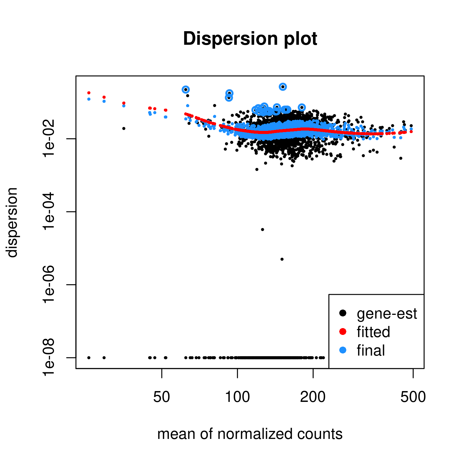
The fitted function has a "hump" meaning that the dispersion becomes higher with the mean for some portion of the graph.
I think that in an RNA-Seq one should be worried if such a graph would be produced. How worrisome is it in ChIP-Seq, in diffbind?
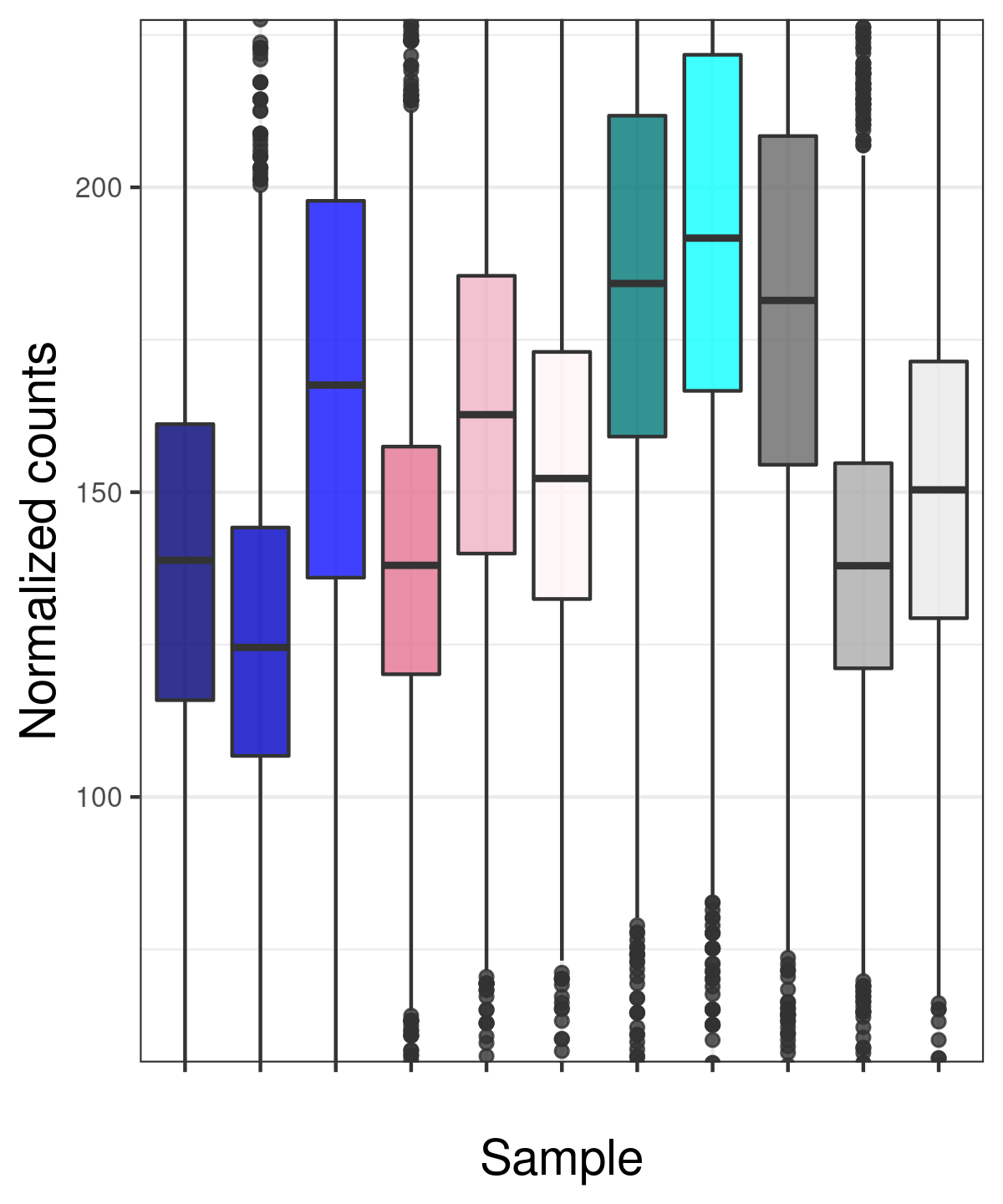
Also, since I cannot assume balanced changes in binding between the various conditions, I have normalized by the total library size - not by DESeq2 native normalization. So unsurprisingly, the distribution is different for the different samples. I think there is no other option - but are these invalidated assumptions that ruin the analysis?
dbObj_b_contrast_qc <- dba.contrast(dbObj_b_norm,design="~Condition")
dbObj_b_res_qc <- dba.analyze(dbObj_b_contrast_qc)
dds_qc <- dba.analyze(dbObj_b_res_qc, bRetrieveAnalysis = T)
plotDispEsts(dds_qc)
normc <- as.data.frame(counts(dds_qc, normalized=T))
myBoxplot(normc) # a function plotting boxplots with ggplot2

print(dds_qc$Condition)
sessionInfo()
Output:
[1] WT         WT         WT         Mut        Mut        Mut
[7] Rescue     Rescue     Rescue_Mut Rescue_Mut Rescue_Mut
Levels: WT Mut Rescue Rescue_Mut


R version 4.0.4 (2021-02-15)
Platform: x86_64-pc-linux-gnu (64-bit)
Running under: Ubuntu 20.04.2 LTS

Matrix products: default
BLAS:   /usr/lib/x86_64-linux-gnu/blas/libblas.so.3.9.0
LAPACK: /usr/lib/x86_64-linux-gnu/lapack/liblapack.so.3.9.0

locale:
 [1] LC_CTYPE=en_IL.UTF-8       LC_NUMERIC=C
 [3] LC_TIME=en_IL.UTF-8        LC_COLLATE=en_IL.UTF-8
 [5] LC_MONETARY=en_IL.UTF-8    LC_MESSAGES=en_IL.UTF-8
 [7] LC_PAPER=en_IL.UTF-8       LC_NAME=C
 [9] LC_ADDRESS=C               LC_TELEPHONE=C
[11] LC_MEASUREMENT=en_IL.UTF-8 LC_IDENTIFICATION=C

attached base packages:
 [1] parallel  stats4    grid      stats     graphics  grDevices utils
 [8] datasets  methods   base

other attached packages:
 [1] limma_3.46.0                rgl_0.105.13
 [3] DiffBind_3.0.13             DESeq2_1.30.1
 [5] SummarizedExperiment_1.20.0 Biobase_2.50.0
 [7] MatrixGenerics_1.2.1        matrixStats_0.58.0
 [9] GenomicRanges_1.42.0        GenomeInfoDb_1.26.2
[11] IRanges_2.24.1              S4Vectors_0.28.1
[13] BiocGenerics_0.36.0         RColorBrewer_1.1-2
[15] pheatmap_1.0.12             ggrepel_0.9.1
[17] ggplot2_3.3.3

loaded via a namespace (and not attached):
  [1] backports_1.2.1          GOstats_2.56.0
  [3] BiocFileCache_1.14.0     plyr_1.8.6
  [5] GSEABase_1.52.1          splines_4.0.4
  [7] crosstalk_1.1.1          BiocParallel_1.24.1
  [9] amap_0.8-18              digest_0.6.27
 [11] htmltools_0.5.1.1        invgamma_1.1
 [13] GO.db_3.12.1             SQUAREM_2021.1
 [15] fansi_0.4.2              magrittr_2.0.1
 [17] checkmate_2.0.0          memoise_2.0.0
 [19] BSgenome_1.58.0          base64url_1.4
 [21] Biostrings_2.58.0        annotate_1.68.0
 [23] systemPipeR_1.24.3       askpass_1.1
 [25] bdsmatrix_1.3-4          prettyunits_1.1.1
 [27] jpeg_0.1-8.1             colorspace_2.0-0
 [29] blob_1.2.1               rappdirs_0.3.3
 [31] apeglm_1.12.0            xfun_0.21
 [33] dplyr_1.0.4              crayon_1.4.1
 [35] RCurl_1.98-1.2           jsonlite_1.7.2
 [37] graph_1.68.0             genefilter_1.72.1
 [39] brew_1.0-6               survival_3.2-7
 [41] VariantAnnotation_1.36.0 glue_1.4.2
 [43] gtable_0.3.0             zlibbioc_1.36.0
 [45] XVector_0.30.0           webshot_0.5.2
 [47] DelayedArray_0.16.1      V8_3.4.0
 [49] Rgraphviz_2.34.0         scales_1.1.1
 [51] mvtnorm_1.1-1            DBI_1.1.1
 [53] edgeR_3.32.1             miniUI_0.1.1.1
 [55] Rcpp_1.0.6               xtable_1.8-4
 [57] progress_1.2.2           emdbook_1.3.12
 [59] bit_4.0.4                rsvg_2.1
 [61] AnnotationForge_1.32.0   truncnorm_1.0-8
 [63] htmlwidgets_1.5.3        httr_1.4.2
 [65] gplots_3.1.1             ellipsis_0.3.1
 [67] farver_2.0.3             pkgconfig_2.0.3
 [69] XML_3.99-0.5             sass_0.3.1
 [71] dbplyr_2.1.0             locfit_1.5-9.4
 [73] utf8_1.1.4               labeling_0.4.2
 [75] manipulateWidget_0.10.1  later_1.1.0.1
 [77] tidyselect_1.1.0         rlang_0.4.10
 [79] AnnotationDbi_1.52.0     munsell_0.5.0
 [81] tools_4.0.4              cachem_1.0.4
 [83] cli_2.3.0                generics_0.1.0
 [85] RSQLite_2.2.3            evaluate_0.14
 [87] stringr_1.4.0            fastmap_1.1.0
 [89] yaml_2.2.1               knitr_1.31
 [91] bit64_4.0.5              caTools_1.18.1
 [93] purrr_0.3.4              RBGL_1.66.0
 [95] mime_0.10                xml2_1.3.2
 [97] biomaRt_2.46.3           compiler_4.0.4
 [99] rstudioapi_0.13          curl_4.3
[101] png_0.1-7                geneplotter_1.68.0
[103] tibble_3.0.6             bslib_0.2.4
[105] stringi_1.5.3            GenomicFeatures_1.42.1
[107] lattice_0.20-41          Matrix_1.3-2
[109] vctrs_0.3.6              pillar_1.5.0
[111] lifecycle_1.0.0          jquerylib_0.1.3
[113] irlba_2.3.3              data.table_1.14.0
[115] bitops_1.0-6             httpuv_1.5.5
[117] rtracklayer_1.50.0       R6_2.5.0
[119] latticeExtra_0.6-29      hwriter_1.3.2
[121] promises_1.2.0.1         ShortRead_1.48.0
[123] KernSmooth_2.23-18       MASS_7.3-53.1
[125] gtools_3.8.2             assertthat_0.2.1
[127] openssl_1.4.3            Category_2.56.0
[129] rjson_0.2.20             withr_2.4.1
[131] GenomicAlignments_1.26.0 batchtools_0.9.15
[133] Rsamtools_2.6.0          GenomeInfoDbData_1.2.4
[135] hms_1.0.0                DOT_0.1
[137] coda_0.19-4              rmarkdown_2.7
[139] GreyListChIP_1.22.0      ashr_2.2-47
[141] mixsqp_0.3-43            bbmle_1.0.23.1
[143] shiny_1.6.0              numDeriv_2016.8-1.1
[145] tinytex_0.29

Thanks. As far as I understand, in CHiP-Seq (unlike RNA-Seq) one can expect major changes between conditions. Whereas expression data has "housekeeping" genes, I think this concept does not apply to protein binding, and one can have large differences resulting from chromatin accessibility. So MA plots (and even their high counts) should not necessarily be on y=0, imho.
Here there is a post which asks "what is the best practice in DiffBind to deal with two data sets that have major changes in chromatin accessibility?". Hopefully the question will be answered there.
That is basically the same. Normalization in these plots seems to be completely off, the OP should focus (as I explained above) on the "arrowhead" regions, as these probably are the most reliable ones. It seems that OP has lots of regions with increased counts in the 2dpr condition and this is setting off normalization. As said I would normalize based on the very highly high-count regions, or try something like bin-based normalization as suggested in the csaw vignette.
This is a good conversation. Normalization of ChIP data is not obvious! While
DiffBindhas several built-in options for normalization options, the best one for your data may require computing the normalization factors outside of the package and then feeding them back in. Other options that would need to be considered upfront is the use of spike-ins, or ChIPing for parallel factors (such as H3K4me3) that work in a similar way to housekeeping genes in RNA-seqI also recommend reading Aaron Lun's discussion of normalization in the
csawuser guide; among other things he talks specifically about trended biases.