QSEA : Internal CNV analysis and cancer type-specific TCGA 450K Human Methylation Calibration Dataset
2
1
Entering edit mode
rtrivedi1 ▴ 10
@4899789e
Last seen 2.8 years ago
United States

Hi everyone,

I am new both to genomic data analysis and R. So my questions may be very basic in nature. Any help will be significant. Thanks in advance ! I have successfully completed QSEA tutorial with given data in MEDIPSData package. However, while using my own data I have few queries.

Similar to example discussed in QSEA package, I am also analyzing MEDIP sequencing data from Tumor (PRAD) and Normal/Control samples. For every tumor and control samples, I have Input Control (IC) alignment bam files. My questions are:

(1) Should I provide IC bam files in the same data frame that have Tumor and Control samples, and do I need to follow specific
nomenclature in group column for IC samples ?

(2) While computing CNV internally from IC, do we need to provide argument "MEDIP = FALSE"? In this case, the addCNV consider fragments with/without CpG dinucleotides ? Is there any resource where addCNV examples with IC have been discussed ? I just want to be sure with the commands I am using to

(3) For TCGA calibration for prostrate cancer, I have downloaded data files TCGA_PRAD_meth450k_level3_wd250.table, TCGA_PRAD_meth450k_level3_wd500.table and TCGA_PRAD_methylation450_level3_beta_values.table from this resource
https://oc-molgen.gnz.mpg.de/owncloud/s/YrQfJnAZLMbTcKb?path=%2F. What processing do I need to perform on these files (.table) to generate 250/500 bp window size-specific .RData output files that can be directly used by QSEA package functions ?

Best Rakesh

MEDIP-seq CNV TCGA450KHumanMethylationCalibrationDataset qsea PRAD • 1.6k views
ADD COMMENT
3
Entering edit mode
@matthias-lienhard-6292
Last seen 3 months ago
Max Planck Institute for molecular Gene…

Hi Rakesh,

To use your input samples for CNV, you need to provide the path to the files in the sample table. The minimal sample table would thus have the following columns:

  • sample_name -> identifier for the sample, make sure to add "normal" or "control" suffix to the healthy tissue control samples (or specify normal_idx parameter in addCNV).
  • file_name -> path to the MeDIP seq bam file
  • input_file_name -> path to the input sample bam file
  • group -> group identifer
  • sex -> male/female this is used to infer the number of sex chromosomes for the calibration of local normalization factors

When calling addCNV, you can now use <<file_name='input_file_name', MeDIP=FALSE>>. You may want to adjust the window_size according to the sequencing depth you have. When setting MeDIP=FALSE all reads are considered, with and without CpG. The parameters for using the MeDIP samples would be <<file_name='file_name', MeDIP=TRUE>>. In this case, only fragments without CpGs are considered.

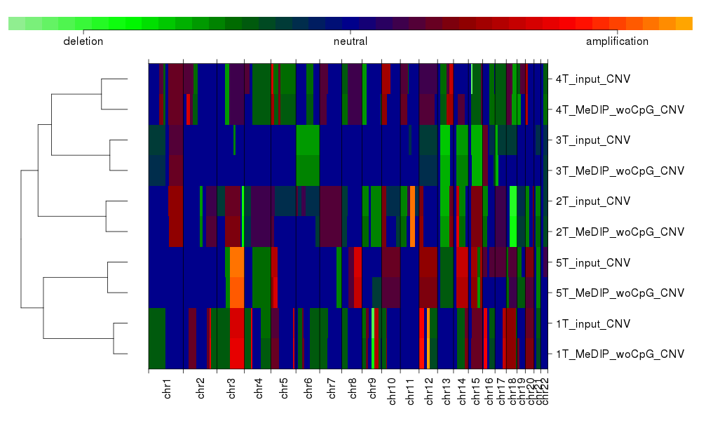
I'd suggest you try both with input seq and MeDIP seq, and compare the result (e.g. the map plotCNV and potentially the primary evidence, that is depicted in the plots you get when setting a plot_dir in addCNV) If you could share this here, it would also be useful to others. In my experience the results should be very similar. This is from the QSEA paper, Supplementary Figure 8:

Comparison of CNV estimates from MeDIP and input seq. Heatmap representation of whole genome CNV profiles for the PDX samples, estimated using MeDIP and input seq. Lines are ordered by hierarchical clustering, based on Euclidian distance between CNV profiles..

The issue with input seq is that it is usually very low coverage (I had less than 1M reads per sample), thus CNVs from MeDIP might actually be more accurate.

ADD COMMENT
0
Entering edit mode

Dear Matthias,

Thank you for the detailed reply to my queries. It is very helpful. As per you suggestion I have prepared my sample table and it looks like this

sample_name file_name   input_file_name group   sex
1T_tumor    1T_5mc.bam  1T_IC.bam       Tumor   male
1N_normal   1N_5mc.bam  1N_IC.bam       Normal  male
2T_tumor    2T_5mc.bam  2T_IC.bam       Tumor   female
2N_normal   2N_5mc.bam  2N_IC.bam       Normal   female
3T_tumor    3T_5mc.bam  3T_IC.bam       Tumor   male
3N_normal   3N_5mc.bam  3N_IC.bam       Normal   male
4T_tumor    4T_5mc.bam  4T_IC.bam       Tumor   female
4N_normal   4N_5mc.bam  4N_IC.bam       Normal   female

I will perform both IC and MedIP samples analysis with window size adjustments if required, and post the results here.

# Command when using input control samples for CNV analysis
qseaSet=addCNV(qseaSet, file_name="input_file_name",window_size=2e6,paired=TRUE, parallel=FALSE, MeDIP=FALSE)

# Command when using MEDIP samples for CNV analysis
qseaSet=addCNV(qseaSet, file_name="file_name",window_size=2e6,paired=TRUE, parallel=FALSE, MeDIP=TRUE)

Thank you again

Best,

Rakesh

ADD REPLY
0
Entering edit mode

Looks good, this should work.

ADD REPLY
3
Entering edit mode
@matthias-lienhard-6292
Last seen 3 months ago
Max Planck Institute for molecular Gene…

Regarding the third point, the data you have downloaded is preprocessed for hg38. In R, you need to import the tabe (which is a tab seperated text file), and optionally parse the ids. You can use the following sniplet (which I adapted from lung cancer, may require changes) to do so:

#infer the classes for faster import
temp=read.table("TCGA_PRAD_meth450k_level3_wd250.table", nrows = 5, header=T, sep="\t", stringsAsFactors=F)
classes <- sapply(temp, class)
classes[1]="character" #the chromosomes
#import the file
tcga_beta_450=read.table("TCGA_PRAD_meth450k_level3_wd250.table", nrows=nr,colClasses = classes, header=T, sep="\t",     stringsAsFactors=F)
names(tcga_beta_450)[1:3]=c("chr", "start", "end")
#import the metadata and match sample ids
tcga_samples=read.table("nationwidechildrens.org_biospecimen_sample_prad.txt", header=T, sep="\t", stringsAsFactors=F)
tcga_samplenames_450=sub("^.+TCGA","TCGA",names(tcga_beta_450)[-(1:3)])
tcga_samplenames_450=sub("\\.0\\dD.+_Beta_value","",tcga_samplenames_450)
tcga_samplenames_450=gsub("\\.","-",tcga_samplenames_450)
m=match(tcga_samplenames_450,tcga_samples$bcr_sample_barcode)
tcga_beta_450=tcga_beta_450[,c(1:3,which(!is.na(m))+3)]
tcga_samplenames_450=tcga_samplenames_450[!is.na(m)]
m=m[!is.na(m)]
tissue=sub("^.+ ","",tcga_samples$sample_type[m])
type=sub("^jhu.usc.edu_","",names(tcga_beta_450)[-(1:3)])
type=sub(".HumanMethylation.+$","",type)

#make sample names like
#TCGA_PRAD_Tumor-66-2794-01A
names(tcga_beta_450)[-(1:3)]=paste0("TCGA_",type,"_",tissue, "_",sub("TCGA-","",tcga_samplenames_450))
names(tcga_beta_450)=gsub("-","_",names(tcga_beta_450))

#find matched pairs (tumor/normal) and sort table accordingly
tumor=grep("Tumor", names(tcga_beta_450))
normal=grep("Normal", names(tcga_beta_450))
m=match(gsub("_?\\d?\\d?[A-Za-z]+(_|$)","",names(tcga_beta_450[tumor])),gsub("_?\\d?\\d?[A-Za-z]+(_|$)","",names(tcga_beta_450[normal])) )
mTumor=tumor[!is.na(m)]
mNormal=normal[m[!is.na(m)]]
paste(names(tcga_beta_450)[mTumor], names(tcga_beta_450)[mNormal] )

save(tcga_beta_450,file=paste0("TCGA_PRAD_450k_samples_250wd_",date,".RData"))

This can now be used for calibration similar as in the tutorial. However, I encorage you to have a good look at the data and choose the parameters accordingly as it seems reasonable to you. For example, what regions you want to consider as fully methylated:

tcga_reg=GRanges(tcga_beta_450$chr, IRanges(tcga_beta_450$start,tcga_beta_450$end))
# suggestion 1: fully methylated is at least 90% methylation in at least 95% of the samples
fullMeth=which(rowSums(tcga_beta_450[,c(tumor, normal)]<.9)<length(c(tumor, normal))*.05)
# suggestion 2: define fully methylated as average >90% and variance<0.05
tcga_means=rowMeans(tcga_beta_450[,c(tumor, normal)])
tcga_var=apply(tcga_beta_450[,c(tumor, normal)],1,var)
#hist(tcga_var)
fullMeth=which(tcga_means>.9 & tcga_var<0.05)

#match the regions
ol=findOverlaps( tcga_reg[fullMeth],getRegions(prad_QSEAset), select="first")
nna=!is.na(ol)
ol=ol[nna]
signal=matrix(tcga_means[fullMeth[nna]],nrow=length(ol), ncol=nrow(getSampleTable(prad_QSEAset)), byrow=F )
prad_QSEAset=addEnrichmentParameters(prad_QSEAset, pattern_name="CpG",signal=signal,windowIdx=ol,bins=seq(.5,40.5,2))
ADD COMMENT
0
Entering edit mode

Dear Matthias,

As you mentioned, I need to make some changes to the sniplet provided by you to generate PRAD-specific RData file that can be used in the QSEA directly. Before that I want to completely understand the steps involved in generation of "tcga_luad_lusc_450kmeth.RData" used in QSEA package. Is there any repository where I can find all the raw files and R scripts to generate "tcga_luad_lusc_450kmeth.Rdata".

Additionally, the sniplet is using input file "nationwidechildrens.org_biospecimen_sample_prad.txt". Is there any specific resource for it or I need to compile specifically for different cancer types.

Thanks

Best, Rakesh

ADD REPLY
0
Entering edit mode

I am not sure what you are referring to by tcga_luad_lusc_450kmeth.Rdata. If you mean the object tcga_luad_lusc_450kmeth, which is part of the example dataset MEDIPSDdata, and used in the calibration, my answer above details out all the steps how it was produced. The nationwidechildrens.org_biospecimen_sample_prad.txt is the clinical information (biospecimen) table you get from tcga data portal. It is anyway only used to set the column names, which is not really required.

The essential steps are: (disclaimer: untested code)

# 1) import the table with the binned methylation values from TCGA
tcga_beta_450=read.table("TCGA_PRAD_meth450k_level3_wd250.table", header=T, sep="\t",     stringsAsFactors=F)
names(tcga_beta_450)[1:3]=c("chr", "start", "end")
# 2) define "fully methylated regions" ( adjust to your needs) 
tcga_means=rowMeans(tcga_beta_450[,-1:3]) # this uses all columns - if you want to select only tumor, you need to adjust the columns selected
tcga_var=apply(tcga_beta_450[,-1:3],1,var)
#hist(tcga_var) #maybe a good idea to look at the distributions to find good thresholds
fullMeth=which(tcga_means>.9 & tcga_var<0.05)
# 3) make a GRange object and match the regions with QSEA regions
tcga_reg=GRanges(tcga_beta_450$chr, IRanges(tcga_beta_450$start,tcga_beta_450$end))
ol=findOverlaps( tcga_reg[fullMeth],getRegions(prad_QSEAset), select="first") #where pradQSEAset is your dataset
nna=!is.na(ol)
ol=ol[nna]
# use the average of the tcga cohort as calibration signal for all your samples:
signal=matrix(tcga_means[fullMeth[nna]],nrow=length(ol), ncol=nrow(getSampleTable(prad_QSEAset)), byrow=F ) samples
# 4) apply the calibration
prad_QSEAset=addEnrichmentParameters(prad_QSEAset, pattern_name="CpG",signal=signal,windowIdx=ol,bins=seq(.5,40.5,2))
ADD REPLY
0
Entering edit mode

Dear Matthias,

Thank you !! With your help I am able to generate PRAD-specific TCGA calibration dataset and it looks something like this:

GRanges object with 6 ranges and 2 metadata columns:
      seqnames        ranges strand | Tumor_mean_methylation Normal_mean_methylation
         <Rle>     <IRanges>  <Rle> |              <numeric>               <numeric>
  [1]     chr1   15751-16000      * |               0.902338                0.905418
  [2]     chr1 533751-534000      * |               0.938074                0.957527
  [3]     chr1 663001-663250      * |               0.931793                0.978342
  [4]     chr1 788751-789000      * |               0.909562                0.925354
  [5]     chr1 791251-791500      * |               0.919957                0.938935
  [6]     chr1 799501-799750      * |               0.935902                0.921397
  -------
  seqinfo: 1 sequence from an unspecified genome; no seqlengths

I am not sure why the seqinfo says "unspecified genome", I have used "BSgenome.Hsapiens.UCSC.hg38" for my studies.

Also, your previous post QSEA: Need help on creating ROI for whole genome MeDIPSeq data to create an annotation file is very helpful.

Thank you again !!

Best,

Rakesh

ADD REPLY
0
Entering edit mode

Hi Rakesh,

the table looks good! The seqinfo is not specified in the GRanges object - which does not matter.

Best, Matthias

ADD REPLY
0
Entering edit mode

Thanks Matthias.

Best

Rakesh

ADD REPLY

Login before adding your answer.

Traffic: 898 users visited in the last hour
Help About
FAQ
Access RSS
API
Stats

Use of this site constitutes acceptance of our User Agreement and Privacy Policy.

Powered by the version 2.3.6