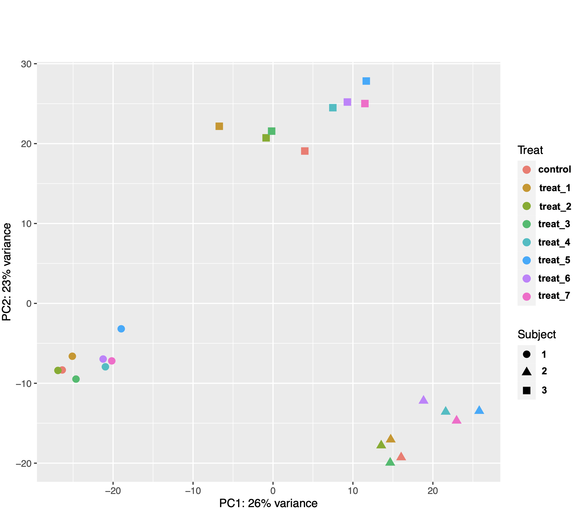
I am using DESeq2 to identify genes that are differentially expressed in mammalian tissue (n = 3 subjects) in response to 8 different treatments in culture. The PCA plot of the samples showed that gene expression was more variable between the biological replicates (subjects) than between treatments (see image below). This made sense biologically because the treatments were applied to subsamples from the same tissue samples from each animal.
I then used the following model design with subject as the blocking factor: design = ~ Subject + Treat. However, after extracting results for my comparisons of interest, I noticed that the number of DEGs was not consistent with the distances between samples on the PCA plot. I know that the gene counts used for PCA are transformed and those used for DE analysis are not, but they still seem really weird.
For example, I got 19 DEG for treat2 vs control, 24 DEG for treat3 vs control, but a whopping106 DEG for treat2 vs treat3. As another example, I got 37 DEG for treat4 vs control, 98 DEG for treat5 vs control, and 128 DEG for treat5 vs treat4. I used control as the reference level for contrasts, so I am wondering if the results function is doing something weird when extracting differences between two non-control treatments. I assumed that contrast = c("Treat", "treat_5, "treat_4") is essentially (treat5 – control) -– (treat4 – control). I get the same results if I use contrast = list("Treat_treat_5_vs_control", "Treat_treat_4_vs_control"). The code I used is below.
dds <- DESeqDataSetFromTximport(txi,
                                colData = samples,
                                design = ~ Subject + Treat)

dds$Treat <- relevel(dds$Treat, ref = "control")

dds <- DESeq(dds)

# example comparisons
res1 <- results(dds, contrast = c("Treat", "treat_5", "control"),
                               alpha = 0.05, pAdjustMethod="BH",
                               lfcThreshold = 1, altHypothesis = "greaterAbs")

res2 <- results(dds, contrast = c("Treat", "treat_5", "treat_4"),
                               alpha = 0.05, pAdjustMethod="BH",
                               lfcThreshold = 1, altHypothesis = "greaterAbs")

# PCA plot
vsd <- vst(dds, fitType="local", blind=FALSE)

pcaData <- plotPCA(vsd, intgroup=c("Treat", "Subject"), returnData=TRUE)

percentVar <- round(100 * attr(pcaData, "percentVar"))

ggplot(pcaData, aes(PC1, PC2, color=Treat, shape=Subject)) +
  geom_point(size=3) +
  xlab(paste0("PC1: ",percentVar[1],"% variance")) +
  ylab(paste0("PC2: ",percentVar[2],"% variance")) +
  coord_fixed()


Agree with swbarnes. The relative number of DEG can't be inferred from the PCA plot in the way you are suggesting.
I recommend looking at plotCounts per gene of interest if you want to investigate DEG results.
Thank you, I will do that!