I am analyzing RNA-seq data, and I have tried both the voom and robustified limma-trend approaches (following the process outlined in RNA-seq analysis is easy as 1-2-3 with limma, Glimma and edgeR and reviewing the user's guide), but the p-values do not agree very well. After adjustment, the robust limma-trend approach results in more significant transcripts than voom, and there is only moderate overlap in what is considered significant by both. The ratio of the largest library size to the smallest is < 1.5, so I don't think it is unreasonable to use limma-trend, though changing the prior.count in cpm() does affect the number of significant features, and I'm not sure what the best offset would be (I use 0.5).
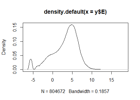
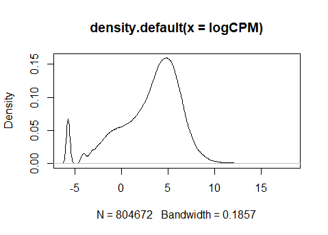
I did notice that the log-cpm values output by each method are a bit different (see below). The first plot uses the log-cpm from voom, and the second uses log-cpm from the cpm() function with prior.count = 0.5:
log-cpm from voom:
log-cpm from cpm(log = TRUE, prior.count = 0.5):
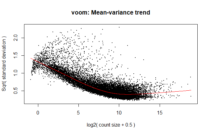
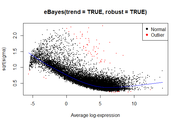
Mean-variance relationship:
I also know that "limma-trend applies the mean-variance relationship at the gene level whereas voom applies it at the level of individual observations" (voom: precision weights unlock linear model analysis tools for RNA-seq read counts), but I don't exactly understand what could be driving the difference in the results, especially when the trend lines are nearly identical.
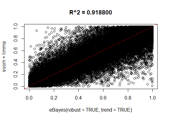
p-value scatterplot:
Below is a scatterplot of the p-values from limma-trend vs the p-values from voom.
It turns out that I had a typo at the very end of my code when I was adjusting p-values across all comparison groups. I had mutate(adj.P.Val = p.adjust(P.Value), "BH") instead of mutate(adj.P.Val = p.adjust(P.Value, "BH")). voomWithQualityWeights (using sample quality weights) now produces results comparable to limma-trend (also using sample quality weights).
In our experience, voom and limma-trend agree well, although obviously they will not be exactly the same otherwise we wouldn't keep both methods. If you think you have a counter example, you would need to provide reproducible code so we can verify that you are applying both methods in equivalent ways.
The p-value correlation you show depends almost entirely on non-significant p-values, so isn't very important in terms of interpretable results. And 0.92 is quite a large correlation anyway. It would be more relevant to compare toptables.
limma-trend is not very sensitive to the cpm prior count, and it will work fine with prior.count=0.5, but we use the default value of prior.count=2. As you might guess, that's why it is set to be the default value.
Thank you for the feedback. While I can't provide the data until it is in the public domain, here is the code that I use. All steps before and after this are the same. I also compared the results of topTable (top 20 features from each contrast tested), and only about 40% of the feature/contrast combinations show up in both tables. This percentage increases to about 54% when comparing the top 1000 features in each contrast.
## Same for both ----
# Create DGEList
dge <- DGEList(counts)

# Filtering features with low counts is not done,
# though it may be a good idea to do so.

# Library size normalization
dge <- calcNormFactors(dge)


## limma-trend ----
# Convert to log CPM
logCPM <- cpm(dge, log = TRUE, prior.count = 2)

# Modeling
fit.smooth <- lmFit(logCPM, design) %>%
    contrasts.fit(contrast.matrix) %>%
    eBayes(trend = TRUE, robust = TRUE)


## voom ----
# Convert to log CPM and calculate observation-level weights
y <- voom(dge, design = design)

# Modeling
fit.smooth <- lmFit(y, design) %>%
    contrasts.fit(contrast.matrix) %>%
    eBayes()
I updated the code so that I am filtering with filterByExpr first and then using robust = TRUE for both methods, but the results are about the same with limma-trend giving about double the number of significant features (though I want to note that the numbers of sig. features are at most in the low double-digits after BH adjustment). I also want to clarify that I missed a set of parentheses when calculating the overlap, and it is actually about 60-80% commonality when I use topTable to compare the top 20-1000 features in each contrast.
Edit: I compared these methods on a different set of contrasts of interest where the number of significant features in each contrast after adjustment approaches 10K, and limma-trend results in only about 2% more significant features and the overlap is at least 96%. Maybe there is just not much difference between the other contrasts of interest, so that lead to the differences in the voom and limma-trend results.


Thank you for the feedback. While I can't provide the data until it is in the public domain, here is the code that I use. All steps before and after this are the same. I also compared the results of topTable (top 20 features from each contrast tested), and only about 40% of the feature/contrast combinations show up in both tables. This percentage increases to about 54% when comparing the top 1000 features in each contrast.