I have samples originating from two tissues (brain and kidney). For a given tissue, I have cancer and normal samples. Brain = 13 (normal = 5 ; cancer = 8) Kidney = 17 (normal = 5 ; cancer = 12)

Goals

1. I want to identifying the DEGs comparing cancer between tissues and normal between tissues. For some patients, I have paired normal-cancer for a given tissue sample.

2. In addition to having confidence in the returned DEGs, I’d like to use the CPM-TMM normalized counts for other analyses outside voom.

Problem: The DEGs are biased for one direction. I don't think this is fully due to the biology.

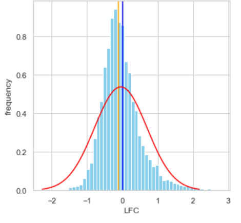
I’m finding that if I take the housekeeping genes as done in the original TMM paper and compute the LFC, I’d expect to see something that’s 0 centered, but I’m seeing a shifter median LFC of -0.1 which for housekeeping genes is clearly wrong. Here, orange line is the observed median; blue, expected median; red line is gaussian with corresponding mean of orange line

Gene Ontology of the returned DEGs yielded what I’d expect with the biology system and what I’ve confirmed with orthogonal analysis methods.

That said, I’m skeptical how attributable this is to the biology vs. technical artifact. And I can’t do analyses with the TMM-adjusted counts.

I'm very stuck for how to proceed.

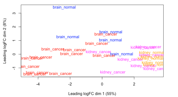
What I’ve done: I observed that I have some outliers on the MDS plot. I eliminated the outlier at (-2, 3) in subsequent analyses. Here’s the MDS plot:

I recognize that the two cancer groups (notably brain_cancer) exhibits high in-group variation. There’s not much I can do about this other than I identified all plausible sources of variation by coloring the points accordingly assessing if I observed any pattern on any of the pairwise combinations of the glMDSPlot, I added it as a covariate to the design matrix.

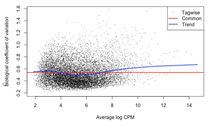
The BCV is 0.54 for the normal and cancer samples. I recognize this is high. The BCV for normal only is 0.34, which is generally consistent with what I’ve read for a BCV of ~0.4.

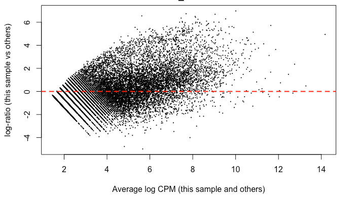
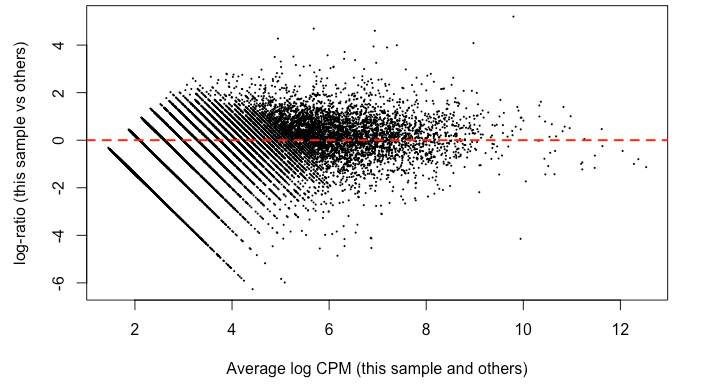
Since it's good practice from the RNAseq , I made MD plots for each sample. In my eyes, this is not zero-centered but rather shifted upwards ~ 2 on the y-axis. This was true of all but two of the samples. Here’s what I mean:

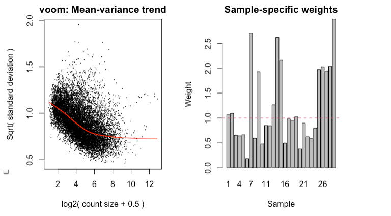
I find it highly alarming that there’s a small, but nonetheless persistent negative median LFC for housekeeping genes. It’s making me not trust the DEG. I tried filtering the CPM cutoff for pre-filtering genes going into the DEG but that didn't materially impact the mean-variance trend which comparing against the online guides doesn't seem too off

Questions: (1) Is there more I can do to address this persistent difference in the cancer samples? I was thinking of recentering all LFC based on the observed median from the HK genes for other comparisons I wanted to make... (2) Are the MD plots shifted or is it just me? (3) Is what I'm concerned about reasonable or is the median I'm worried about normal? I’m relatively new to voom, read a lot of documentation. I did not use voom() together with eBayes(trend=TRUE). I'm using voomWithQualityWeights given the ratio of the max to min library size. I tried filtering gene expression a priori as described in the Chen et al 2016 guide.

Thank you for creating such a well-document tool and supporting it. I learned from all the posts I read.

Code (if it's helpful):

counts <- read.csv(paste0("../", countsf), header = TRUE, row.names = 1)

meta <- read.csv(paste0("../", metaf),
                 header = TRUE)

dge <- dge[keep, , keep.lib.sizes = FALSE]
dge <- calcNormFactors(dge, method = 'TMM')

design <- model.matrix(~0 + meta$tissue + meta$disease_status+ meta$input_rna +  meta$seq_batch + meta$sample_id, data = meta)

vwts <- voomWithQualityWeights(counts = dge, 
                               design = design,
                               normalize.method = 'none',
                               method = "genebygene",
                               plot=TRUE) 

corfit <- duplicateCorrelation(vwts, design, block = meta$sample_id)

vwts <- voomWithQualityWeights(counts = dge,
                               design = design,
                               normalize.method = 'none',

                               method = "genebygene",
                               block = meta$sample_id,
                               correlation = corfit$consensus,
                               plot=TRUE) 
corAgain <- duplicateCorrelation(vwts, design, block = meta$sample_id)

vfit2 <- lmFit(vwts, design,
               block = meta$sample_id,
               correlation = corfit$consensus)

cm <- makeContrasts(
  brain_cancer_normal = brain_cancer - brain_normal,
  kidney_cancer_normal = kidney_cancer - kidney_normal,
  levels = colnames(design)
)

vfit3 <- contrasts.fit(vfit2, cm)
vfit3 <- eBayes(vfit3, trend = FALSE, robust = TRUE) 
vfit3_decideTests <- decideTests(vfit3, method = "global", p.value = 0.05)

If you want a stronger normalization, then set normalize.method to "quantile" or "cyclicloess". Either of those normalization methods are much stronger than scale normalization like TMM.

You are analysing RNA-seq data with absolutely huge differences between and within groups. It's hard to imagine groups that would be more different than brain vs kidney or normal vs cancer. Moreover the samples are likely to be highly variable in terms of quality and there are likely to be a variety of batch effects. With data like this, the plots are never going to look pretty. At the same time, the differences between the groups are so marked that it is not necessary to have low variability in order to detect the main differences reliably.

There is no biological or statistical reason why log-fold-changes should be centered on zero and TMM makes no such assumption. Who shouldn't there be more up genes than down genes? Personally, I do not believe in the existence of "housekeeping genes" whose expression should always be the same, especially between such radically different tissues as brain cancer and kidney cancer.

Please do not recenter the log-fold-changes. There's no justification for ad hoc tinkering like that. Better to use quantile normalization.